R luncheon 3

Lesson Outline

Vector data
Simple features
Creating spatial data with simple features
Basic geospatial analysis

Welcome to the third R luncheon! By popular demand, the final two luncheons will explore using R as a GIS. Today’s session will focus on geospatial analysis using the new simple features package and our final session will focus on creating publication ready maps in R. We will focus entirely on working with vector data in these next two lessons, but checkout the raster and rgdal packages if you want to work with raster data in R. There are several useful vignettes in the raster link.

Please note that this is not an introduction to R and you are also expected to have an understanding of basic geospatial concepts for these next two sessions. You can visit any of the other topics on our main page for a refresher on some of the R basics. In the mean time, feel free to ask plenty of questions as we go through today’s lesson!

The goals for today are:

Understand the vector data structure
Understand how to import and structure vector data in R
Understand how R stores spatial data using the simple features package
Execute basic geospatial functions in R

Vector data

Most of us should already be familiar with the basic types of spatial data and their components. We’re going to focus entirely on vector data for this lesson because these data are easily conceptualized as features or discrete objects with spatial information. We’ll discuss some of the details about this later. Raster data by contrast are stored in a regular grid where the cells of the grid are associated with values. Raster data are more common for data with continuous coverage, such as climate or weather layers.

Vector data come in three flavors. The simplest is a point, which is a 0-dimensional feature that can be used to represent a specific location on the earth, such as a single tree or an entire city. Linear, 1-dimensional features can be represented with points (or vertices) that are connected by a path to form a line and when many points are connected these form a polyline. Finally, when a polyline’s path returns to its origin to represent an enclosed space, such as a forest, watershed boundary, or lake, this forms a polygon.

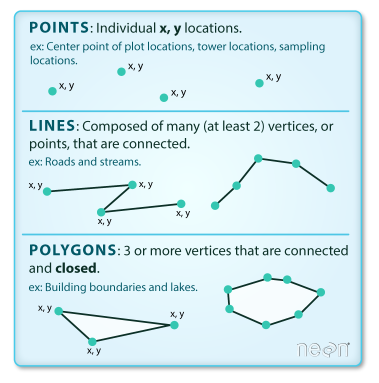
https://earthdatascience.org/courses/earth-analytics/spatial-data-r/intro-vector-data-r/

Image source

All vector data are represented similarly, whether they’re points, lines or polygons. Points are defined by a single coordinate location, whereas a line or polygon is several points with a grouping variable that distinguishes one object from another. In all cases, thishe aggregate dataset is composed of one or more features of the same type (points, lines, or polygons).

There are two other pieces of information that are included with vector data. The attributes that can be associated with each feature and the coordinate reference system or CRS. The attributes can be any supporting information about a feature, such as a text description or summary data about the features. You can identify attributes as anything in a spatial dataset that is not explicitly used to define the location of the features.

The CRS is used to establish a frame of reference for the locations in your spatial data. The chosen CRS ensures that all features are correctly referenced relative to each other, especially between different datasets. As a simple example, imagine comparing length measurements for two objects where one was measured in centimeters and another in inches. If you didn’t know the unit of measurement, you could not compare relative lengths. The CRS is similar in that it establishes a common frame of reference, but for spatial data. An added complication with spatial data is that location can be represented in both 2-dimensional or 3-dimensional space. This is beyond the scope of this lesson, but for any geospatial analysis you should be sure that:

the CRS is the same when comparing datasets, and
the CRS is appropriate for the region you’re looking at.

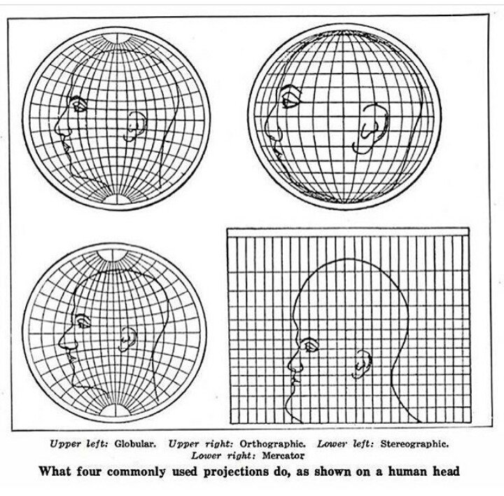
Image source

To summarize, vector data include the following:

spatial data (e.g., latitude, longitude) as points, lines, or polygons
attributes
a coordinate reference system

These are all the pieces of information you need to recognize in your data when working with features in R.

Simple features

R has a long history of packages for working with spatial data. For many years, the sp package was the standard and most widely used toolset for working with spatial data in R. This package laid the foundation for creating spatial data classes and methods in R, but unfortunately it’s development predated a lot of the newer tools that are built around the tidyverse. This makes it incredibly difficult to incorporate sp data objects with these newer data analysis workflows.

The simple features or sf package was developed to streamline the use of spatial data in R and to align its functionality with those provided in the tidyverse. The sf package is already beginning to replace sp as the fundamental spatial model in R for vector data. A major advantage of sf, as you’ll see, is its intuitive data structure that retains many familiar components of the data.frame (or more accurately, tibble).

Simple Features is a hierarchical data model that represents a wide range of geometry types - it includes all common vector geometry types (but does not include raster) and even allows geometry collections, which can have multiple geometry types in a single object. From the first sf package vignette we see:

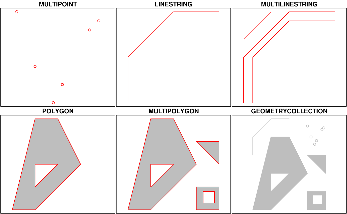
You’ll notice that these are the same features we described above, with the addition of “multi” features and geometry collections that include more than one type of feature.

Creating spatial data with simple features

Let’s get setup for today:

Open RStudio and create a new project.
In the new project directory, create a folder called “data”.
Download this zipped folder to your computer (anywhere) and copy its contents to the “data” folder in your project.
From the file menu, open a new script within the project. At the top of the script, install the sf package if you haven’t done so and load the package after installation.

install.package('sf')
library(sf)

After the package is loaded, you can check out all of the methods that are available for sf data objects. Many of these names will look familiar if you’ve done geospatial analysis before. We’ll use some of these a little bit later.

methods(class = 'sf')

##  [1] $<-                   [                     [[<-                 
##  [4] aggregate             anti_join             arrange              
##  [7] as.data.frame         cbind                 coerce               
## [10] dbDataType            dbWriteTable          distinct             
## [13] filter                full_join             gather               
## [16] group_by              identify              initialize           
## [19] inner_join            left_join             merge                
## [22] mutate                nest                  plot                 
## [25] print                 rbind                 rename               
## [28] right_join            sample_frac           sample_n             
## [31] select                semi_join             separate             
## [34] show                  slice                 slotsFromS3          
## [37] spread                st_agr                st_agr<-             
## [40] st_as_sf              st_bbox               st_boundary          
## [43] st_buffer             st_cast               st_centroid          
## [46] st_collection_extract st_convex_hull        st_coordinates       
## [49] st_crs                st_crs<-              st_difference        
## [52] st_geometry           st_geometry<-         st_intersection      
## [55] st_is                 st_line_merge         st_node              
## [58] st_point_on_surface   st_polygonize         st_precision         
## [61] st_segmentize         st_set_precision      st_simplify          
## [64] st_snap               st_sym_difference     st_transform         
## [67] st_triangulate        st_union              st_voronoi           
## [70] st_wrap_dateline      st_write              st_zm                
## [73] summarise             transmute             ungroup              
## [76] unite                 unnest               
## see '?methods' for accessing help and source code

All of the functions and methods in sf are prefixed with st_, which stands for ‘spatial and temporal’. This is kind of confusing but this is in reference to standard methods avialable in PostGIS, an open-source backend that is used by many geospatial platforms. An advantage of this prefixing is all commands are easy to find with command-line completion in sf, in addition to having naming continuity with existing software.

There are two ways to create a spatial data object in R, i.e., an sf object, using the sf package.

Directly import a shapefile
Convert an existing R object with latitude/longitude data that represent point features

We’ll import a shapefile first and look at its structure so we can better understand the sf object. The st_read() function can be used for import. Setting quiet = T will keep R from being chatty when it imports the data.

polys <- st_read('data/Bight13_MPAs_Offshore.shp', quiet = T)
polys

## Simple feature collection with 25 features and 2 fields
## geometry type:  MULTIPOLYGON
## dimension:      XY
## bbox:           xmin: 182769 ymin: 3599568 xmax: 488069.6 ymax: 3818896
## epsg (SRID):    26911
## proj4string:    +proj=utm +zone=11 +datum=NAD83 +units=m +no_defs
## First 10 features:
##           Region      MPA_Name                       geometry
## 1   Campus Point  Campus Point MULTIPOLYGON (((238555.2 38...
## 2         Naples        Naples MULTIPOLYGON (((230453.5 38...
## 3      Kashtayit     Kashtayit MULTIPOLYGON (((205345.2 38...
## 4   Abalone Cove  Abalone Cove MULTIPOLYGON (((372581.6 37...
## 5  Point Vicente Point Vicente MULTIPOLYGON (((366154.7 37...
## 6     Point Dume    Point Dume MULTIPOLYGON (((333051.1 37...
## 7     Point Dume    Point Dume MULTIPOLYGON (((331883.2 37...
## 8     Dana Point    Dana Point MULTIPOLYGON (((430436.8 37...
## 9   Laguna Beach  Laguna Beach MULTIPOLYGON (((426176.2 37...
## 10  Laguna Beach  Laguna Beach MULTIPOLYGON (((425246.4 37...

What does this show us? Let’s break it down.

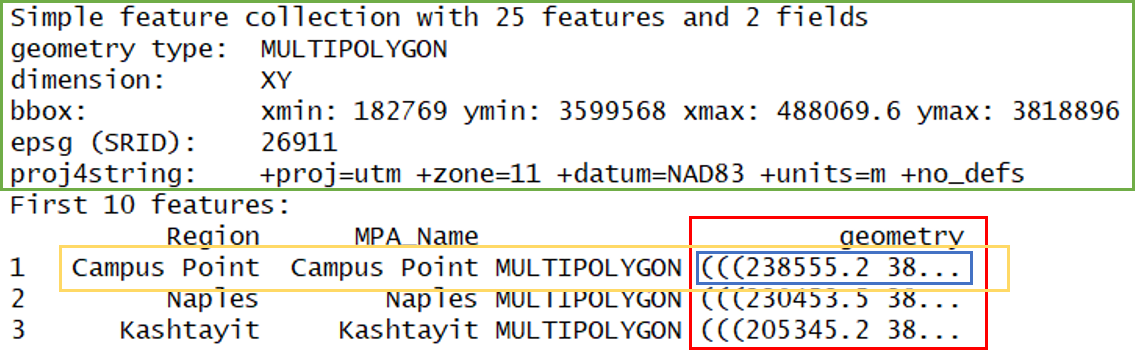
In green, metadata describing components of the sf object
In yellow, a simple feature: a single record, or data.frame row, consisting of attributes and geometry
In blue, a single simple feature geometry (an object of class sfg)
In red, a simple feature list-column (an object of class sfc, which is a column in the data.frame)

We’ve just imported a multipolygon dataset with 25 features and 2 fields. The dataset is projected using the UTM Zone 11 CRS. You’ll notice that the actual dataset looks very similar to a regular data.frame, with some interesting additions. The header includes some metadata about the sf object and the geometry column includes the actual spatial information for each feature. Conceptually, you can treat the sf object like you would a data.frame.

Easy enough, but what if we have point data that’s not a shapefile? You can create an sf object from any existing data.frame so long as the data include coordinate information (e.g., columns for longitude and latitude) and you know the CRS (or can make an educated guess). Let’s first import a dataset from a .csv file.

stations <- read.csv('data/AllBightStationLocations.csv', stringsAsFactors = F)
str(stations)

## 'data.frame':    1772 obs. of  4 variables:
##  $ StationID: chr  "1001" "1003" "1005" "1014" ...
##  $ Bight    : int  1994 1994 1994 1994 1994 1994 1994 1994 1994 1994 ...
##  $ Latitude : num  34 34 34 34 34 ...
##  $ Longitude: num  -119 -119 -119 -119 -118 ...

The st_as_sf() function can be used to make this data.frame into a sf object, but we have to tell it which column is the x-coordinates and which is the y-coordinates. We also have to specify a CRS - this is just a text string or number (i.e, EPSG) in a standard format for geospatial data. A big part of working with spatial data is keeping track of reference systems between different datasets. Remember that meaningful comparisons between datasets are only possible if the CRS is shared.

There are many, many types of reference systems and plenty of resources online that provide detailed explanations of the what and why behind the CRS (see spatialreference.org or this guide from NCEAS). For now, just realize that we can use a simple text string in R to indicate which CRS we want. Although this may not always be true, we can make an educated guess that the standard geographic projection with the WGS84 datum applies to our dataset.

stations <- stations %>% 
  st_as_sf(coords = c('Longitude', 'Latitude'), crs = '+proj=longlat +ellps=WGS84 +datum=WGS84 +no_defs')

Now we can see the data in full sf glory.

stations

## Simple feature collection with 1772 features and 2 fields
## geometry type:  POINT
## dimension:      XY
## bbox:           xmin: -120.6092 ymin: 32.04718 xmax: -117.0871 ymax: 34.46742
## epsg (SRID):    4326
## proj4string:    +proj=longlat +datum=WGS84 +no_defs
## First 10 features:
##    StationID Bight                   geometry
## 1       1001  1994 POINT (-118.6077 33.98533)
## 2       1003  1994    POINT (-118.569 33.984)
## 3       1005  1994  POINT (-118.5373 33.9825)
## 4       1014  1994 POINT (-118.5588 33.97417)
## 5       1019  1994   POINT (-118.48 33.97067)
## 6       1025  1994  POINT (-118.476 33.96833)
## 7       1026  1994   POINT (-118.4965 33.967)
## 8       1027  1994 POINT (-118.5138 33.94867)
## 9       1028  1994 POINT (-118.5882 33.96583)
## 10       103  1994 POINT (-120.1839 34.42055)

These two datasets describe some relevant information about our Bight sampling program. The stations data includes all locations that have been sampled from 1993 to 2013 and the polys data show locations of marine protected areas (MPAs) in the Bight. We might be interested in knowing which stations occur in MPAs, how many stations, or when they were sampled. We can address all of these questions in R, but before we proceed we need to make sure the two datasets share a CRS. We can check this with st_crs().

st_crs(polys)

## Coordinate Reference System:
##   EPSG: 26911 
##   proj4string: "+proj=utm +zone=11 +datum=NAD83 +units=m +no_defs"

st_crs(stations)

## Coordinate Reference System:
##   EPSG: 4326 
##   proj4string: "+proj=longlat +datum=WGS84 +no_defs"

You’ll have to choose one of the reference systems to use as the common format. Either one will work but sometimes it’s better to go with the UTM format since it references location using actual units of measurement, i.e., meters. This can make spatial analyses simpler, such as estimating areas or spatial overlap between datasets. The st_transform() function can be used to transform an existing CRS for an sf obect to another.

stations <- stations %>% 
  st_transform(crs = st_crs(polys))

We can verify that both are now projected to UTM zone 11.

st_crs(polys)

## Coordinate Reference System:
##   EPSG: 26911 
##   proj4string: "+proj=utm +zone=11 +datum=NAD83 +units=m +no_defs"

st_crs(stations)

## Coordinate Reference System:
##   EPSG: 26911 
##   proj4string: "+proj=utm +zone=11 +datum=NAD83 +units=m +no_defs"

Basic geospatial analysis

As with any analysis, let’s take a look at the data to see what we’re dealing with before we start comparing the two.

plot(stations)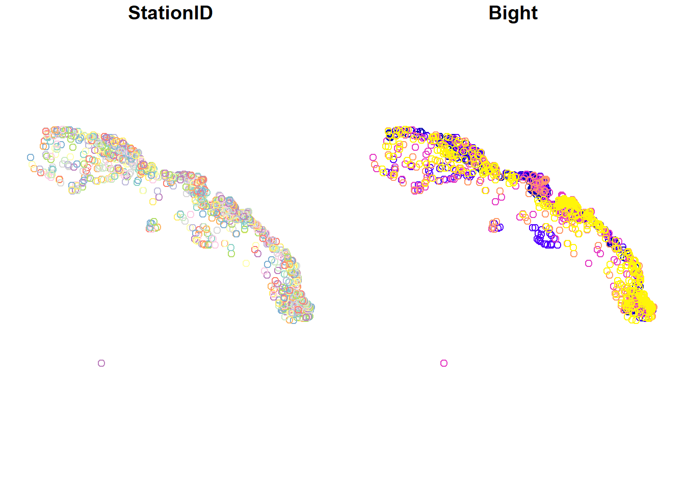

plot(polys)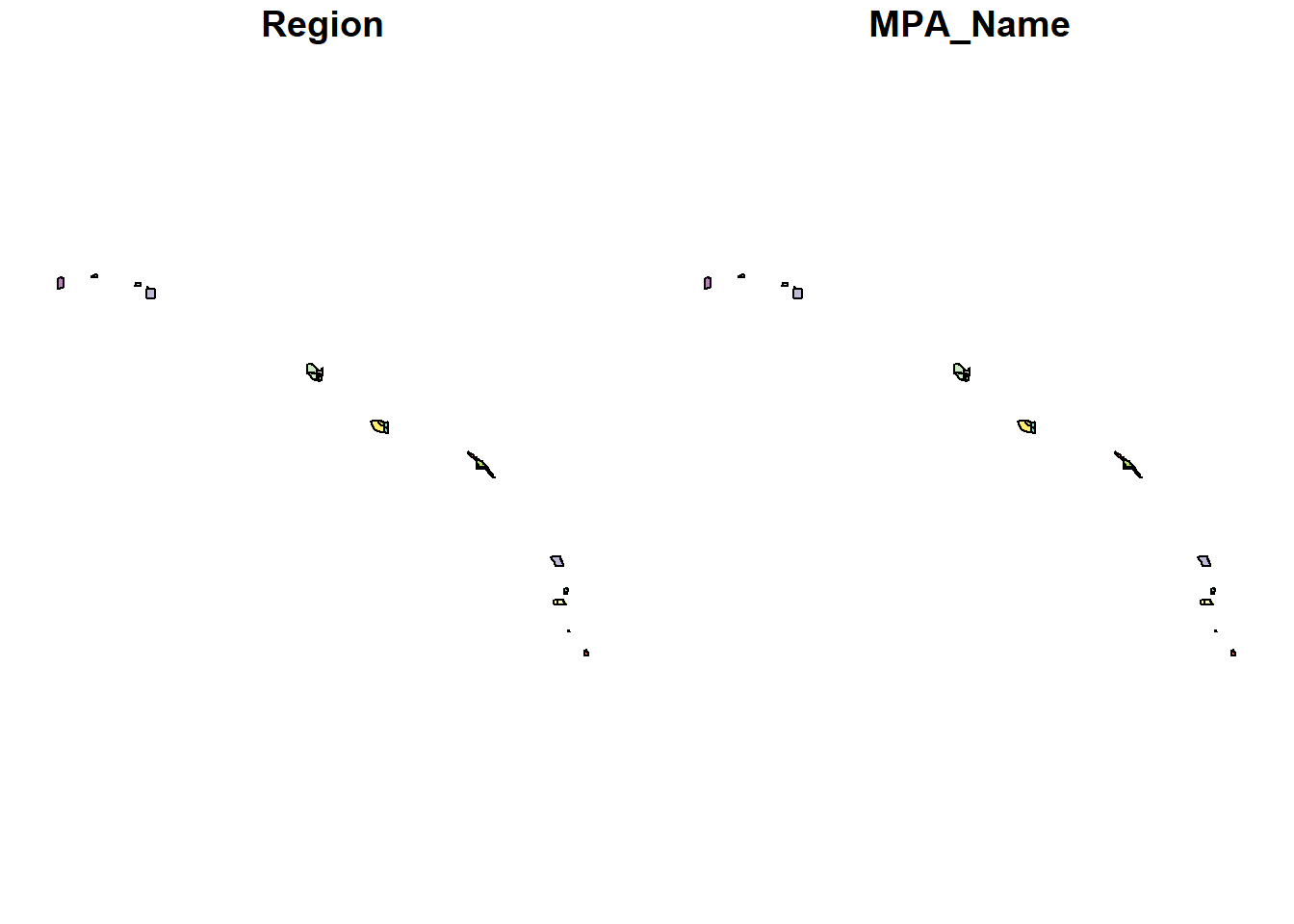

So we have lots of stations and only a handful of MPAs. You’ll also notice that the default plotting method for sf objects is to create one plot per attribute feature. This is intended behavior but sometimes is not that useful (it can also break R if you have many attributes). Maybe we just want to see where the data are located independent of any of the attributes. We can accomplish this by plotting only the geometry of the sf object.

plot(stations$geometry)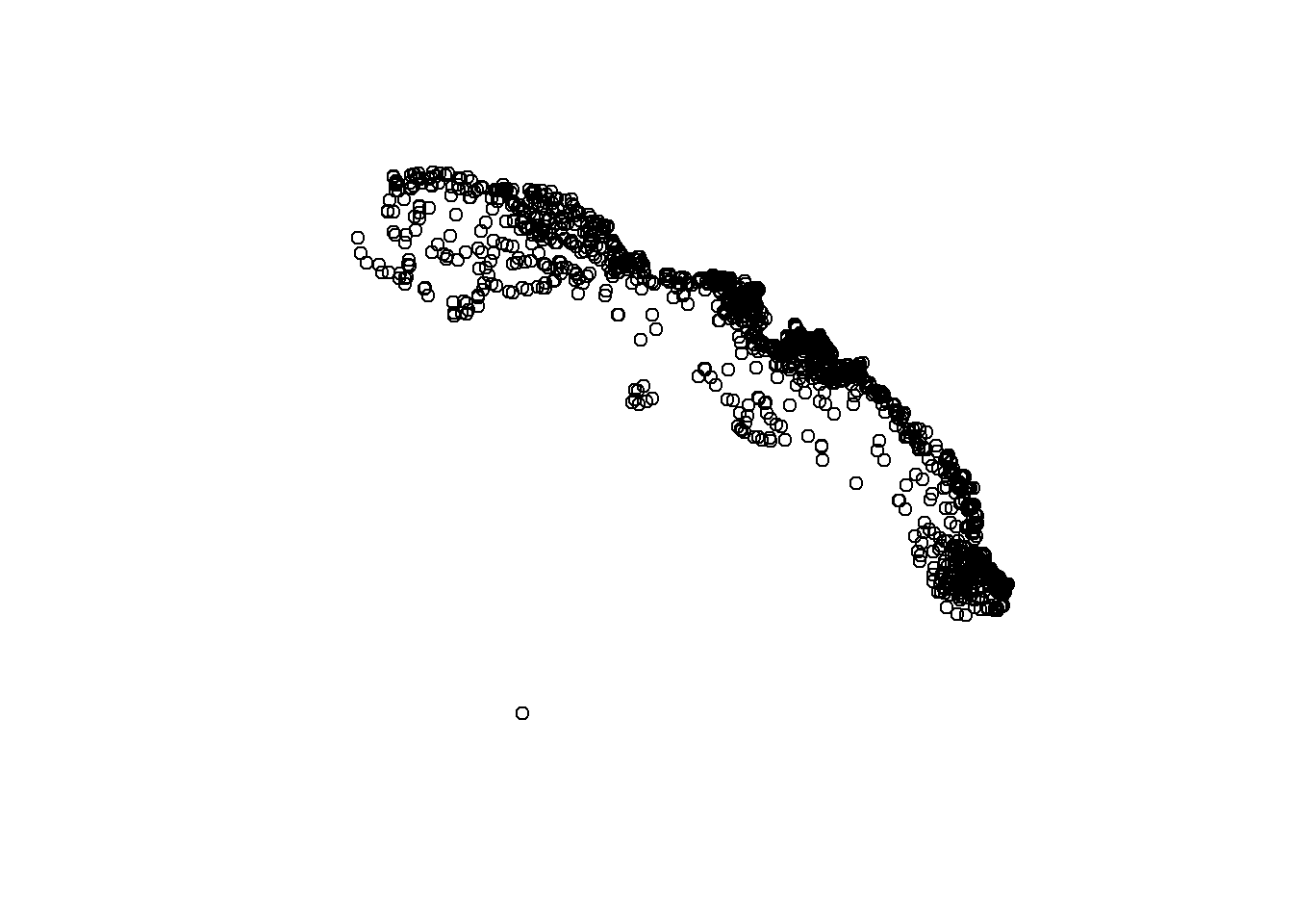

plot(polys$geometry)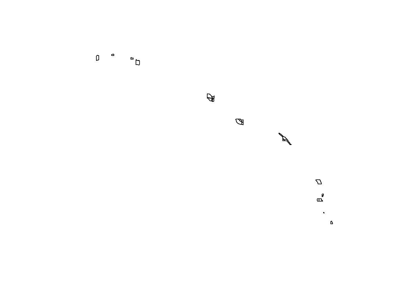

To emphasize the point that the sf package plays nice with the tidyverse, let’s do a simple filter on the stations data using the dplyr package to get only the stations that were sampled 2013.

filt_dat <- stations %>% 
  filter(Bight == 2013)
plot(filt_dat$geometry)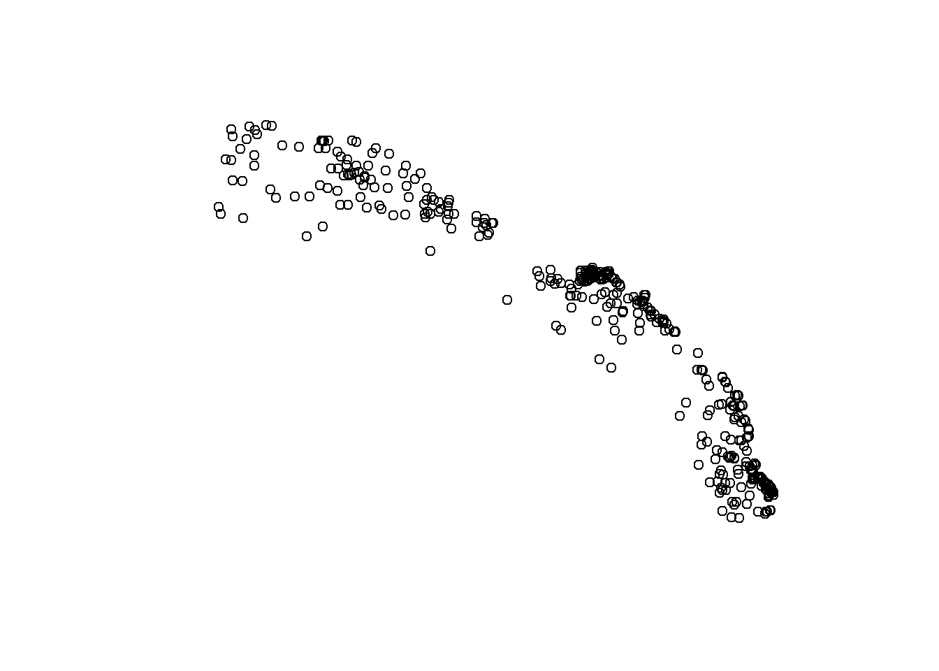

Now let’s use the stations (all years) and MPA polygons to do a quick geospatial analysis. Our simple question is:

How many stations were sampled in each MPA and in which year?

The first task is to subset the stations data (all years) by locations on the Bight that are MPAs. There are a few ways we can do this. The first is to make simple subset where we filter the station locations using a spatial overlay with the MPA polygons. The second and more complete approach is to intersect the two data objects to subset and combine the attributes.

stat_sub <- stations[polys, ]
plot(stat_sub$geometry)

stat_sub

## Simple feature collection with 78 features and 2 fields
## geometry type:  POINT
## dimension:      XY
## bbox:           xmin: 185052.3 ymin: 3600023 xmax: 486783 ymax: 3818682
## epsg (SRID):    26911
## proj4string:    +proj=utm +zone=11 +datum=NAD83 +units=m +no_defs
## First 10 features:
##     StationID Bight                 geometry
## 63       1214  1994 POINT (368981.1 3732850)
## 124      1739  1994 POINT (475988.5 3637071)
## 127      1769  1994 POINT (469244.9 3629514)
## 250       988  1994   POINT (333960 3762522)
## 339      2201  1998   POINT (370970 3732041)
## 406      2277  1998 POINT (428939.3 3707890)
## 407      2278  1998 POINT (429085.2 3707523)
## 408      2279  1998 POINT (428852.5 3708723)
## 409      2280  1998 POINT (428586.9 3707971)
## 423      2294  1998 POINT (471527.9 3651705)

With this first approach we can see which stations were located in an MPA, but we don’t know the name of the MPA for each station. A better approach is to use st_intersection to both overlay and combine the attribute fields from the two data objects.

stat_sub <- st_intersection(stations, polys)
plot(stat_sub$geometry)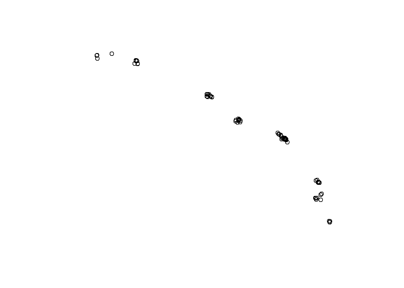

stat_sub

## Simple feature collection with 78 features and 4 fields
## geometry type:  POINT
## dimension:      XY
## bbox:           xmin: 185052.3 ymin: 3600023 xmax: 486783 ymax: 3818682
## epsg (SRID):    26911
## proj4string:    +proj=utm +zone=11 +datum=NAD83 +units=m +no_defs
## First 10 features:
##      StationID Bight       Region     MPA_Name                 geometry
## 477       2359  1998 Campus Point Campus Point POINT (236647.1 3810051)
## 478       2360  1998 Campus Point Campus Point POINT (235656.7 3809592)
## 1366      7735  2008 Campus Point Campus Point POINT (236686.3 3810041)
## 1742  B13-9454  2013 Campus Point Campus Point POINT (237928.3 3805676)
## 1743  B13-9455  2013 Campus Point Campus Point POINT (234072.3 3805918)
## 1744  B13-9456  2013 Campus Point Campus Point POINT (237958.9 3805845)
## 1749  B13-9465  2013 Campus Point Campus Point POINT (237201.6 3809665)
## 1751  B13-9467  2013 Campus Point Campus Point POINT (236647.1 3810051)
## 1752  B13-9468  2013 Campus Point Campus Point POINT (235726.9 3810228)
## 1772  B13-9488  2013    Kashtayit    Kashtayit POINT (204510.8 3818682)

Now we can easily see which Bight sampling stations and years were in which MPA polygon. We can use some familiar tools from dplyr to get the aggregate counts of stations by years in each MPA using the sf object.

stat_cnt <- stat_sub %>% 
  group_by(MPA_Name, Bight) %>% 
  summarise(
    cnt = n()
  ) 
stat_cnt

## Simple feature collection with 33 features and 3 fields
## geometry type:  GEOMETRY
## dimension:      XY
## bbox:           xmin: 185052.3 ymin: 3600023 xmax: 486783 ymax: 3818682
## epsg (SRID):    26911
## proj4string:    +proj=utm +zone=11 +datum=NAD83 +units=m +no_defs
## # A tibble: 33 x 4
## # Groups:   MPA_Name [14]
##    MPA_Name     Bight   cnt                                       geometry
##    <fct>        <int> <int>                                 <GEOMETRY [m]>
##  1 Abalone Cove  1998     1                         POINT (370970 3732041)
##  2 Campus Point  1998     2 MULTIPOINT (235656.7 3809592, 236647.1 381005~
##  3 Campus Point  2008     1                       POINT (236686.3 3810041)
##  4 Campus Point  2013     6 MULTIPOINT (234072.3 3805918, 235726.9 381022~
##  5 Crystal Cove  1998     1                       POINT (422982.1 3713411)
##  6 Crystal Cove  2013     4 MULTIPOINT (419406.6 3716022, 420497.1 371461~
##  7 Dana Point    2003     1                       POINT (430217.1 3706920)
##  8 Dana Point    2008     1                       POINT (430018.1 3706927)
##  9 Dana Point    2013     2 MULTIPOINT (429995.1 3707036, 431557.4 370410~
## 10 Kashtayit     2013     1                       POINT (204510.8 3818682)
## # ... with 23 more rows

Notice that we’ve retained the sf data structure in the aggregated dataset but the structure is now slightly different, both in the attributes and the geometry column. MPA polygons with more than one station within a year have been aggregated to multipoint objects and our cnt column shows the number of stations that make up the aggregation. This is a really powerful feature of sf: spatial attributes are retained during the wrangling process.

We can also visualize this information with ggplot2.

library(ggplot2)
ggplot(stat_cnt, aes(x = MPA_Name, y = cnt)) + 
  geom_bar(stat = 'identity')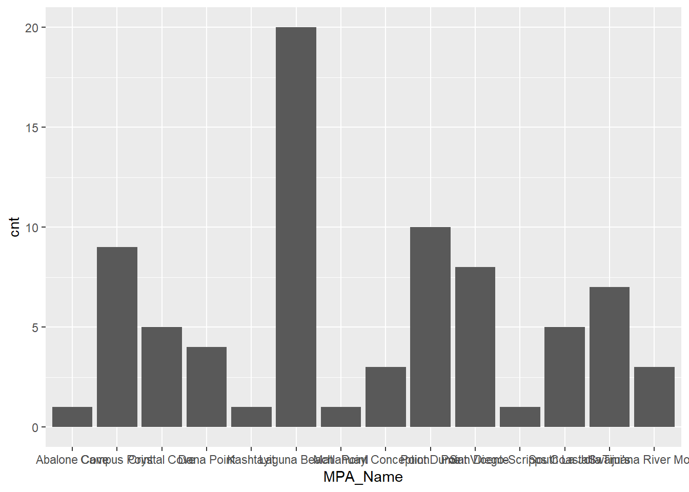

Let’s make it more readable by facetting the plot by sample year and flipping the axes.

ggplot(stat_cnt, aes(x = MPA_Name, y = cnt)) + 
  geom_bar(stat = 'identity') + 
  facet_wrap(~Bight) + 
  coord_flip()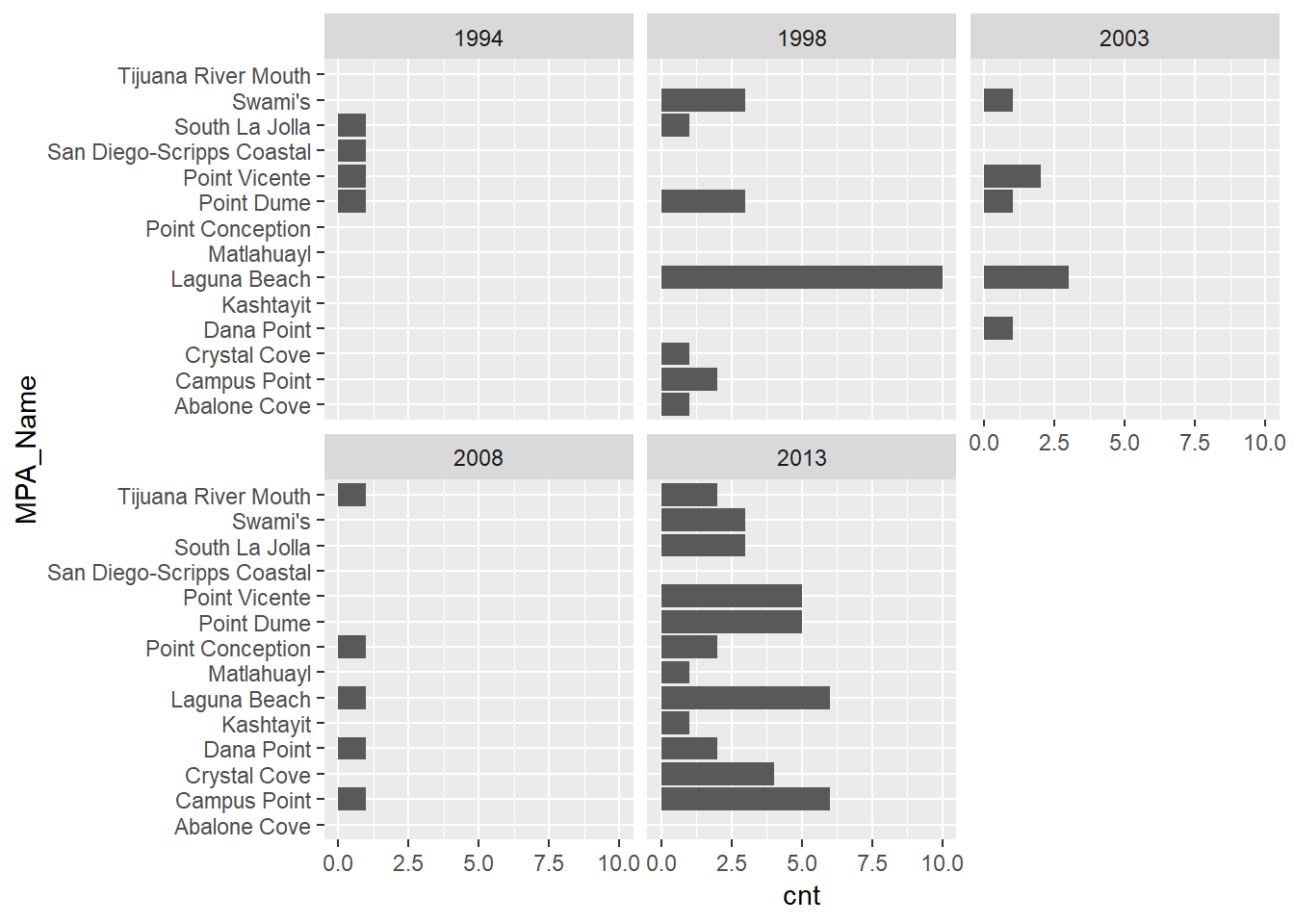

We can see a clear increase in the number of MPAs that were sampled with more recent Bight sampling years. Keep in mind that these data are still sf objects and we can leverage some of the mapping tools in R to spatially view these results. Using the mapview package, we can easily create an interactive map of the MPA polygons and the intersected stations from stat_sub. We’ll cover this in more detail next time but here’s a quick teaser.

library(mapview)
mapview(polys) +
  mapview(stat_sub, zcol = 'Bight')

Excercise

Let’s repeat the above example but instead of spatially aggregating sample locations by MPA we’ll aggregate by sediment characteristics. To accomplish this, we’ll import the sediment chemistry dataset, join it with our sample locations, and aggregate the chemistry data by MPA. We’ll end up with an average concentration of some sediment data for each MPA.

Import the sediment chemistry data into R from the data folder using read_excel() from the readxl package. This file is called data/B13 Chem data.xlsx.
From the chemistry data:
- select() the Year, StationID, Parameter, and Result columns.
- Use filter() to get only the rows in Year that are equal to 2013. Then use filter() again to get rows for the Parameter column that are equal to Arsenic (hint: filter(chemdat, Year == 2013 & Parameter == 'Arsenic')
- Use rename() to rename the Year column to Bight. This will let you join the chemistry data with our stations data.
Using our stat_sub dataset created above, use inner_join() to join stat_sub with the chemistry data. Then use select() to select only the StationID and Result columns from the joined dataset.
Now use st_join() to spatially join the MPA polygon dataset to the joined chemistry/stations dataset (hint: polyjn <- st_join(polys, chemjn)).
Then use the joined polygon dataset for the aggregation of the sediment chemistry data. Use group_by(MPA_Name) to establish a grouping variable, then summarise the Result column with summarise() to take the average arsenic values by each MPA (hint: summarise(Result = mean(Result, na.rm = T))).
Use mapview to plot the polygons and the argument zcol = 'Result' to show the average arsenic in each MPA.

# import and wrangle sediment chemistry
library(readxl)
chemdat <- read_excel('data/B13 Chem data.xlsx') %>% 
  select(Year, StationID, Parameter, Result) %>% 
  filter(Year == 2013 & Parameter == 'Arsenic') %>% 
  rename(Bight = Year)

# join sediment chemistry with stat_sub from above
chemjn <- inner_join(stat_sub, chemdat, by = 'StationID') %>% 
  select(StationID, Result)

# spatially join the MPA polygon data to the joined chemistry/stations data
# aggregate the results by the average
polyjn <- st_join(polys, chemjn) %>% 
  group_by(MPA_Name) %>% 
  summarise(Result = mean(Result, na.rm = T)) 
  
# plot  
mapview(polyjn, zcol = 'Result')