Introduction to R
Lesson Outline
Lesson Exercises
Goals and Motivation
R is a language for statistical computing as well as a general purpose programming language. Increasingly, it has become one of the primary languages used in data science and for data analysis across many of the natural sciences.
We only have two hours to introduce basic concepts in R. I’s an unrealistic expectation that you will be competent after only two hours. As such, the goals of this training are to expose you to fundamentals and to develop an appreciation of what’s possible with this software. I also want to provide resources that you can use for follow-up learning on your own.
You should be able to answer these questions at the end of this session:
- What is R and why should I use it?
- Why would I use RStudio and RStudio projects?
- How can I write, save, and run scripts in RStudio?
- Where can I go for help?
- What are the basic data structures in R?
- How do I import/export data?
Why should I invest time in R?
There are many programming languages available and each has it’s specific benefits. R was originally created as a statistical programming language but now it is largely viewed as a ‘data science’ language. Why would you invest time in learning R compared to other languages?
- The growth of R as explained in the Stack Overflow blog, IEEE rating
R is also an open-source programming language - not only is it free, but this means anybody can contribute to it’s development. As of 2018-10-03, there are 13085 on CRAN!
Python is another popular open-source programming language. Many beginners often ask the quesiton, why R vs. Python? This is an interesting debate with no easy answer. Some things to consider:
- R has statistical roots, phython does not
- Pick the language that has the tools you need, but…
- You can accomplish very similar things with both
Some cool things you can do with R:
- Serious data ninjery
- Graphics and interaction, accidental aRt
- Reproducible research
RStudio
In the old days, the only way to use R was directly from the Console - this is a bare bones way of running R only with direct input of commands. Now, RStudio is the go-to Interactive Development Environment (IDE) for R. Think of it like a car that is built around an engine. It is integrated with the console and includes many other features such as version control, debugging, dynamic documents, package manager and creation, and code highlighting and completion.
Let’s get familiar with RStudio before we go on.
Open R and RStudio
Find the RStudio shortcut and fire it up (just watch for now). You should see something like this:
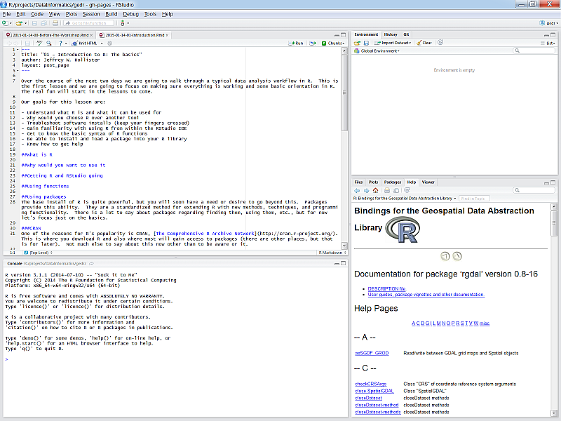
There are four panes in RStudio:
- Source
- console
- Environment, History, etc.
- Files, plots, etc.
RStudio projects
I strongly encourage you to use RStudio projects when you are working with R. The RStudio project provides a central location for working on a particular task. It helps with file management and is portable if all the files live in the same file tree. RStudio projects also remember history - what commands you used and what data objects are in your enviornment.
To create a new project, click on the File menu at the top and select ‘New project…’
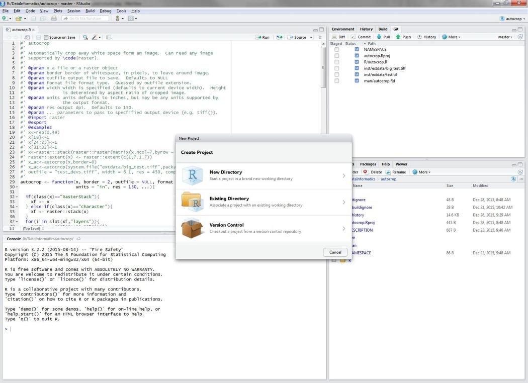
It’s ofen hard to determine the scope of a project. When should a new project be created Should one project be used for a dissertation? Probably not. What about one project for manipulating one data file? Probably not. To help you determine the scope of each project, think about these questions:
- What is the purpose of using R right now?
- Am I manipulating multiple files?
- Are all these files linked by a common theme (e.g., abundance data, environmental data)
- If I shared this with someone, would they have all the necessary data?
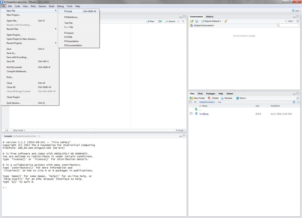
Scripting
In most cases, you will not enter and execute code directly in the console. Code can be created in a script and then sent directly to the console when you’re ready to run it. The key difference here is that a script can be saved and shared.
Open a new script from the File menu…
Executing code in RStudio
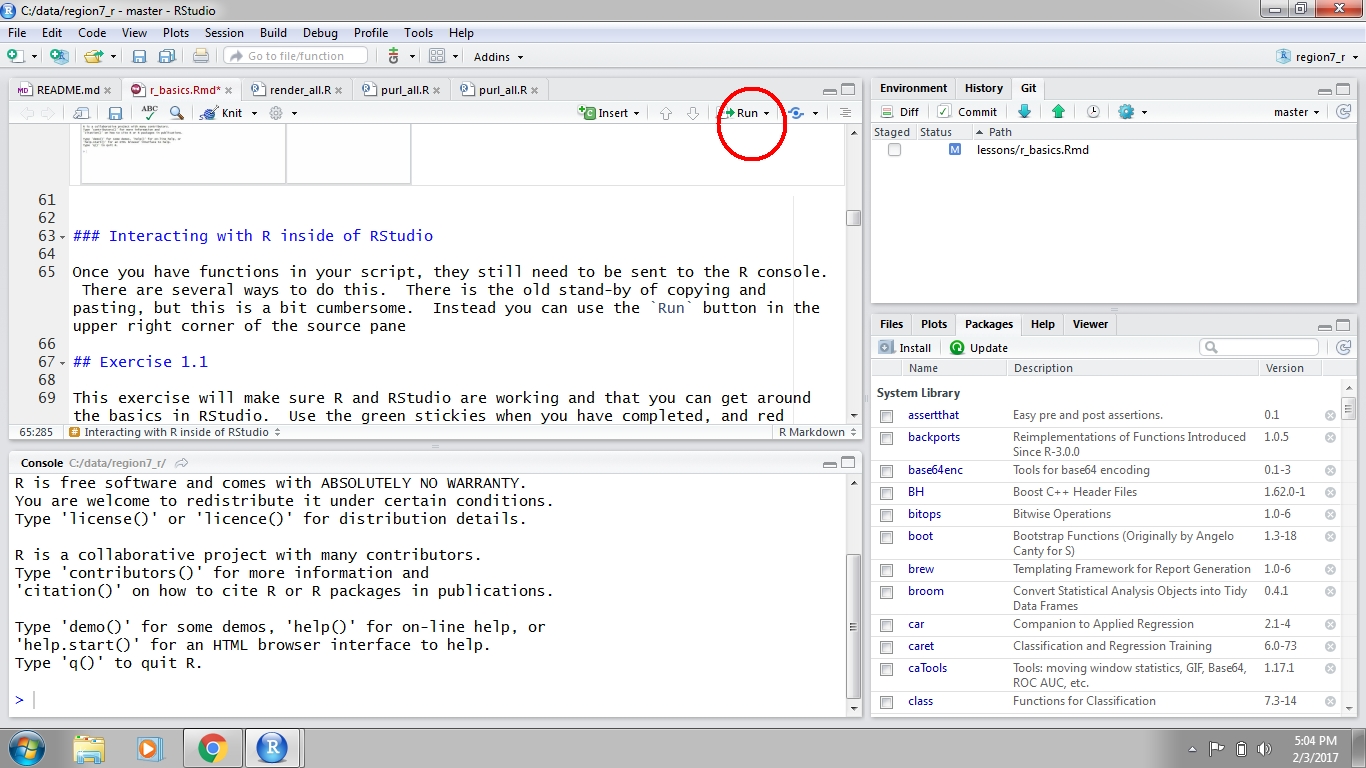
After you write your script it can be sent to the Console to run the code in R. Any variables you create in your script will not be available in your working environment until this is done. There are two ways to sent code the console. First, you can hit the Run button at the top right of the scripting window. Second, and preferred, you can use ctrl+enter. Both approaches will send the selected line to the console, then move to the next line. You can also highlight and send an entire block of code.
What is the environment?
There are two outcomes when you run code. First, the code will simply print output directly in the console. Second, there is no output because you have stored it as a variable (we’ll talk about variable assignment later). Output that is stored is actually saved in the environment. The environment is the collection of named objects that are stored in memory for your current R session. Anything stored in memory will be accessible by it’s name without running the original script that was used to create it.
Exercise 1
This exercise will make sure R and RStudio are working and that you can get around the basics in RStudio. Use the blue stickies when you have completed, and red stickies if you are running into problems.
Start RStudio: To start both R and RStudio requires only firing up RStudio. RStudio should be available from All Programs at the Start Menu. Fire up RStudio.
Take a few minutes to look around RStudio. Find the Console Pane. Find Global and Project Options (hint: look in Tools). Look at the Environment, History Pane. Look at the Files, Plots, Packages, etc. pane.
Create a new project. Name it “sccwrp_r_workshop”. We will use this for the rest of the workshop.
Create a new “R Script” in the Source Pane, save that file into your newly created project and name it “sccwrp_r_workshop.R”. It’ll just be a blank text file at this point.
Add in a comment line to separate this section. It should look something like:
# Exercise 1: Just Getting used to RStudio and Scripts.Add a single line to this script with the following text:
ls(). This is an R function that lists objects in your current environment. Use the various ways we showed to send this command to the R Console. Also, try typing this directly into the R Console and hitEnterto run it.Lastly, we need to get this project set up with some example data for our upcoming exercises. You should have downloaded this already, but if not, the data are available from https://github.com/SCCWRP/R_training_2018/raw/master/lessons/data/mpg.xlsx. Create a folder in your new project named
dataand copy this file into this location.
R language fundamentals
The basic syntax of a function follows the form: function_name(arg1, arg2, ...).
With the base install, you will gain access to many (3389 functions, to be exact). Some examples:
# print
print('hello world!')
## [1] "hello world!"# sequence
seq(1, 10)## [1] 1 2 3 4 5 6 7 8 9 10# random numbers
rnorm(100, mean = 10, sd = 2)## [1] 8.531921 11.905716 11.251795 8.438629 9.450414 8.486819 10.243004
## [8] 12.274041 10.197025 9.520608 10.810758 9.679102 9.111759 6.899313
## [15] 10.932673 10.462370 6.201299 10.577593 6.452287 8.660075 12.135389
## [22] 8.532985 9.595898 11.824422 10.982700 8.463049 10.586093 13.374349
## [29] 10.224231 8.950736 10.206238 8.819724 10.955189 11.149782 10.684488
## [36] 10.969980 9.696980 11.157332 12.117536 9.367518 12.061794 9.272101
## [43] 9.030856 11.227226 10.945037 8.741399 10.144285 11.247540 11.113333
## [50] 9.996750 10.336736 11.890317 10.467867 10.887259 13.292540 8.956129
## [57] 12.559586 9.987806 9.995999 10.420017 11.839114 13.113262 13.162324
## [64] 12.080590 8.458970 10.615528 6.484628 11.538441 5.998108 11.641810
## [71] 7.355314 12.231942 13.406046 8.572844 6.931587 9.148484 10.668048
## [78] 10.992527 9.660655 8.273125 9.018200 8.453254 10.173665 10.900872
## [85] 8.383527 14.767823 6.640291 9.962048 12.812723 6.779957 12.000798
## [92] 11.496873 11.315262 10.184519 10.602588 9.054141 10.566485 7.039364
## [99] 8.111413 9.423223# average
mean(rnorm(100))## [1] -0.04246624# sum
sum(rnorm(100))## [1] -2.929205Very often you will see functions used like this:
my_random_sum <- sum(rnorm(100))In this case the first part of the line is the name of an object. You make this up. Ideally it should have some meaning, but the only rules are that it can’t start with a number and must not have any spaces. The second bit, <-, is the assignment operator. This tells R to take the result of sum(rnorm(100)) and store it an object named, my_random_sum. It is stored in the environment and can be used by just executing it’s name in the console.
my_random_sum## [1] 6.390332With this, you have the very basics of how we write R code and save objects that can be used later.
A few side notes
Sometimes you might see a variable assignment using the = sign:
my_random_sum = sum(rnorm(100))While technically this is the same as <-, it’s generally considered poor practice in code writing. The = sign in R is typically reserved for arguments within functions:
rnorm(100, mean = 10, sd = 1)You might also see these guys in R code:
#Denotes a comment, anything after this on the same line is not run by the console. You can use as many####as you like. Always comment your code and err on the side of too much!()These will almost always be used with functions.[]These are used for indexing values from a stored variable, e.g., I want to see the fifth value in a variable that is 100 numbers long.{}These are used to create your own function or when a chunk of code is meant to be run together.
"or'are used to identify characters in R, they mean the same thing but they do not mix!
Packages
The base install of R is quite powerful, but you will soon have a need or desire to go beyond this. Packages provide this ability. They are a standardized method for extending R with new methods, techniques, and programming functionality. There is a lot to say about packages regarding finding them, using them, etc., but for now let’s focus just on the basics.
CRAN
One of the reasons for R’s popularity is CRAN, The Comprehensive R Archive Network. This is where you download R and also where most will gain access to packages (there are other places, but that is for later). Not much else to say about this now other than to be aware of it. As of 2018-10-03, there are 13085 on CRAN!
Installing packages
When a package gets installed, that means the source is downloaded and put into your library. A default library location is set for you so no need to worry about that. In fact on Windows most of this is pretty automatic. Let’s give it a shot.
#Installing Packages from CRAN
# Install dplyr and ggplot2
install.packages("ggplot2")
install.packages("dplyr")

# You can also put more than one in like
install.packages(c("quickmapr","formatR"))
Packages only need to be installed one time, unless you’re updating to a newer version.
Using packages
One source of confusion that many have is when they cannot access a package that they just installed. This is because getting to this point requires an extra step, loading (or attaching) the package.
# Loading packages into your library
# Add libraries to your R Session
library("ggplot2")
library("dplyr")

# You can also access functions without loading by using package::function
dplyr::mutate
## function (.data, ...)
## {
## UseMethod("mutate")
## }
## <bytecode: 0x00000000182037a0>
## <environment: namespace:dplyr>You will often see people use require() to load a package. It is better form to not do this. For a more detailed explanation of why library() and not require() see Yihui Xie’s post on the subject
And now for a little pedantry. You will often hear people use the terms “library” and “package” interchangeably. This is not correct. A package is what is submitted to CRAN, it is what contains a group of functions that address a common problem, and it is what has allowed R to expand. A library is, more or less, where you packages are stored. You have a path to that library and this is where R puts new packages that you install (e.g. via install.packages()). These two terms are related, but most certainly different. Apologies up front if I slip and use one when I actually mean the other…
You can see where your library is located:
.libPaths()## [1] "C:/Users/Marcus.SCCWRP2K/R/win-library/3.5"
## [2] "C:/Program Files/R/R-3.5.1/library"There are a few ways to see if a package is installed, and if installed, if it’s loaded in your environment (i.e, if you’ve forgot). RStudio makes this easy with it’s user interface (Packages tab, Environment tab), but I encourage you to learn the functions that do this for you. Especially…
# check if a package is installed
"dplyr" %in% installed.packages()

# check if it's loaded
sessionInfo()
Getting Help
Being able to find help and interpret that help is probably one of the most important skills for learning a new language. R is no different. Help on functions and packages can be accessed directly from R, can be found on CRAN and other official R resources, searched on Google, found on StackOverflow, or from any number of fantastic online resources. I will cover a few of these here.
Help from the console
Getting help from the console is straightforward and can be done numerous ways.
# Using the help command/shortcut
# When you know the name of a function
help("print") # Help on the print command
?print # Help on the print command using the `?` shortcut

# When you know the name of the package
help(package = "dplyr") # Help on the package `dplyr`

# Don't know the exact name or just part of it
apropos("print") # Returns all available functions with "print" in the name
??print # shortcut, but also searches demos and vignettes in a formatted page
Official R Resources
In addition to help from within R itself, CRAN and the R-Project have many resources available for support. Two of the most notable are the mailing lists and the task views.
- R Help Mailing List: The main mailing list for R help. Can be a bit daunting and some (although not most) senior folks can be, um, curmudgeonly…
- R-sig-ecology: A special interest group for use of R in ecology. Less daunting than the main help with participation from some big names in ecological modelling and statistics (e.g., Ben Bolker, Gavin Simpson, and Phil Dixon).
- Environmetrics Task View: Task views are great in that they provide an annotated list of packages relevant to a particular field. This one is maintained by Gavin Simpson and has great info on packages relevant to much of the work at EPA.
- Spatial Analysis Task View: One I use a lot that lists all the relevant packages for spatial analysis, GIS, and Remote Sensing in R.
Google and StackOverflow
While the resources already mentioned are useful, often the quickest way is to just turn to Google. However, a search for “R” is a bit challenging. A few ways around this. Google works great if you search for a given package or function name. You can also search for mailing lists directly (i.e. “R-sig-geo”), although Google often finds results from these sources.
Blind googling can require a bit of strategy to get the info you want. Some pointers:
- Always preface the search with “r”
- Understand which sources are reliable
- Take note of the number of hits and date of a web page
- When in doubt, search with the exact error message
One specific resource that I use quite a bit is StackOverflow with the ‘r’ tag. StackOverflow is a discussion forum for all things related to programming. You can then use this tag and the search functions in StackOverflow and find answers to almost anything you can think of. However, these forums are also very strict and I typically use them to find answers not to ask questions.
### Other Resources
As I mentioned earlier, there are TOO many resources to list here and everyone has their favorites. Below are just a few that I like.
- R For Cats: Basic introduction site, meant to be a gentle and light-hearted introduction
- Advanced R: Web home of Hadley Wickham’s new book. Gets into more advanced topics, but also covers the basics in a great way.
- CRAN Cheatsheets: A good cheat sheet from the official source
- RStudio Cheatsheets: Additional cheat sheets from RStudio. I am especially fond of the data wrangling one.
Data structures in R
Now that you know how to get started in R and where to find resources, we can begin talking about R data structures. Simply put, a data structure is a way for programming languages to handle information storage.
There is a bewildering amount of formats for storing data and R is no exception. Understanding the basic building blocks that make up data types is essential. All functions in R require specific types of input data and the key to using functions is knowing how these types relate to each other.
Vectors (one-dimensional data)
The basic data format in R is a vector - a one-dimensional grouping of elements that have the same type. These are all vectors and they are created with the c function:
dbl_var <- c(1, 2.5, 4.5)
int_var <- c(1L, 6L, 10L)
log_var <- c(TRUE, FALSE, T, F)
chr_var <- c("a", "b", "c")
The four types of atomic vectors (think atoms that make up a molecule aka vector) are double (or numeric), integer, logical, and character. For most purposes you can ignore the integer class, so there are basically three types. Each type has some useful properties:
class(dbl_var)## [1] "numeric"length(log_var)## [1] 4These properties are useful for not only describing an object, but they define limits on which functions or types of operations that can be used. That is, some functions require a character string input while others require a numeric input. Similarly, vectors of different types or properties may not play well together. Let’s look at some examples:
# taking the mean of a character vector
mean(chr_var)

# adding two numeric vectors of different lengths
vec1 <- c(1, 2, 3, 4)
vec2 <- c(2, 3, 5)
vec1 + vec2
Coercion
By definition, vectors contain elements of the same type. Combining a vector with different types will coerce elements to the more flexible type. This is intentional behavior of R that makes it easier to combine different data types from a programmatic perspective. In theory, you do not need to combine elements of different types in the same vector because a vector should describe one piece of information (e.g., abundance counts of fish at different sites are always described with numbers).
# combining a character and numeric
c('a', 1)
## [1] "a" "1"Coercion can sometimes create unintentional headaches so just be aware that this happens when you try to combine different data types. R will typically send a warning to the console if information is lost with coercion.
2-dimensional data
A collection of vectors represented as a single data object are often described as two-dimensional data. The simplest case is a matrix that is simply a collection of vectors all of the same type.
# a matrix of characters
mymat <- matrix(letters, ncol = 13)
dim(mymat)
## [1] 2 13# a matrix of numerics
mymat <- matrix(1:12, ncol = 4)
dim(mymat)## [1] 3 4Note that now the matrix has a dim attribute that describes the number of rows and columns in the data. The data that a matrix contains is of course limited to one type. This has limitations, but it can be an efficient fore storing lots of information. You’ll probably encounter matrices if you plan on doing community-level analysis, e.g., abundance data where each row represent a site and each column is a species.
A more common way of storing two-dimensional data is in a data frame (i.e., data.frame). As you probably guessed, these are similar to a matrix with the added bonus of combining data of different types. Think of them like your standard spreadsheet, where each column describes a variable and rows link observations between columns. Here’s a simple example:
ltrs <- c('a', 'b', 'c')
nums <- c(1, 2, 3)
logs <- c(T, F, T)
mydf <- data.frame(ltrs, nums, logs)
mydf
## ltrs nums logs
## 1 a 1 TRUE
## 2 b 2 FALSE
## 3 c 3 TRUEA data frame has other attributes that are not included in a matrix, such as row names and column names. These are useful for indexing (selecting) different parts of the data. (more about this below).
names(mydf)## [1] "ltrs" "nums" "logs"row.names(mydf)## [1] "1" "2" "3"As you might have guessed, a requirement of a matrix or data frame is that all columns have the same number of rows. You can combine vectors wtih different lengths using the list structure. In fact, a data frame is simply a special case of a list where all the vectors have the same length (try as.list(mydf)).
# create a simple list
ltrs <- c('a', 'b', 'c')
nums <- c(1, 2, 3, 4)
myls <- list(ltrs, nums)
myls
## [[1]]
## [1] "a" "b" "c"
##
## [[2]]
## [1] 1 2 3 4Lists have the least constraints on the types of data that can be stored and therefore are the most flexible of the two-dimensional structures. In fact, you can create an n-dimensional list by creating lists of lists, lists of list of lists, etc. List elements are also not limited to vectors and can include any kind of data object (e.g., model output). You will probably not use them a lot in your early R adventures, but they are a very powerful option for data storage.
Data I/O
Input
It is the rare case when you manually enter your data in R. Most data analysis workflows typically begin with importing a dataset from an external source. Literally, this means committing a dataset to memory (i.e., storing it as a variable) as one of R’s data structure formats.
If you’re lucky, your data are already in a flat, rectangular format. In other words, your data are two-dimensional as standard ASCI text. Flat data files present the least complications on import because there is very little to assume about the structure of the data. On import, R tries to guess the data type for each column and this is fairly unambiguous with flat files. The base installation of R comes with some easy to use functions for importing flat files, such as read.table() and read.csv.
More often you will probably have an Excel spreadsheet to import. This is not a preferred format but the reality is that most people are using this software for data storage. In the old days, importing spreadsheets into R was almost impossible given the proprietary data structure of Excel. The tools available in R have since matured and it’s now pretty painless to import a spreadsheet. But “painless” comes with some caveats.
You will save yourself a lot of trouble with data import from Excel if you think like a machine. Consider the example below:
Computers, although very trainable, are also very dumb. If you have trouble interpreting the information, can you expect a computer to do so? Most issues importing Excel spreadsheets relate to format of the data. Here are few pointers to keep in mind if you are using Excel to store data:
- Use the one spreadsheet, one data frame rule (rectangular)
- No colors or special formatting
- No links between sheets
- One data type per column
- Use simple column names (no spaces or special characters)
- Be explicit and consistent with missing values
Following these simple guidelines will make import much, much smoother.
The readxl package is the most recent and by far most flexible data import package for Excel files. It comes with the tidyverse family of packages (more about this next training), but you can install it separately as follows:
install.packages('readxl')Once installed, we can load it to access the import functions.
library(readxl)We’ll import the mpg dataset that describes fuel economy of different car models. This dataset actually comes with R but I’ve saved it as a an Excel spreadsheet to demonstrate the read_excel import function. If you haven’t downloaded the file already, grab it from the online materials and save it in your data folder in your project.
Now we can import the file (note the relative path):
dat <- read_excel('data/mpg.xlsx')If you didn’t get any errors or warnings, the file is now stored in your environment.
ls()## [1] "all_pipes" "alldat" "bad_ex"
## [4] "bad_ex2" "bsmap" "by_make"
## [7] "by_yr_drv" "chemdat" "chr_var"
## [10] "cols" "dat" "dat_ext"
## [13] "datchem" "datlocs" "dbl_var"
## [16] "displ_cat" "dplyr_arr" "dplyr_good_fuel"
## [19] "dplyr_mut" "dplyr_mut2" "dplyr_rnm"
## [22] "dplyr_sel1" "dplyr_sel2" "dplyr_sel3"
## [25] "dplyr_six_cyl" "filt1" "filt2"
## [28] "filt3" "filt4" "filt5"
## [31] "good_ex" "int_var" "log_var"
## [34] "logs" "ltrs" "metadat"
## [37] "more_sums" "mpg" "my_random_sum"
## [40] "mydf" "myls" "mymat"
## [43] "nums" "origin" "p"
## [46] "pkgs" "polys" "prm"
## [49] "sedchem" "stations" "sumdat"
## [52] "tidydat" "x"Before we go on, let’s look at the data class:
class(dat)## [1] "tbl_df" "tbl" "data.frame"head(dat)## # A tibble: 6 x 11
## manufacturer model displ year cyl trans drv cty hwy fl class
## <chr> <chr> <dbl> <dbl> <dbl> <chr> <chr> <dbl> <dbl> <chr> <chr>
## 1 audi a4 1.80 1999. 4. auto~ f 18. 29. p comp~
## 2 audi a4 1.80 1999. 4. manu~ f 21. 29. p comp~
## 3 audi a4 2.00 2008. 4. manu~ f 20. 31. p comp~
## 4 audi a4 2.00 2008. 4. auto~ f 21. 30. p comp~
## 5 audi a4 2.80 1999. 6. auto~ f 16. 26. p comp~
## 6 audi a4 2.80 1999. 6. manu~ f 18. 26. p comp~The data are in the tibble format. A tibble is basically a data frame with some extra features, mostly related to how the data are printed in the console. You’ll encounter tibbles a lot if you are using the tidyverse family of packages, which we’ll go over next training. There are some very good reasons to use tibbles for data wrangling but they can also cause some headaches when used with other packages. For now, let’s just coerce the tibble to a data frame.
dat <- as.data.frame(dat)
class(dat)
## [1] "data.frame"Now let’s look at the data to get an idea of the structure:
# get the dimensions
dim(dat)
## [1] 234 11# get the column names
names(dat)## [1] "manufacturer" "model" "displ" "year"
## [5] "cyl" "trans" "drv" "cty"
## [9] "hwy" "fl" "class"# get the row names
row.names(dat)## [1] "1" "2" "3" "4" "5" "6" "7" "8" "9" "10" "11"
## [12] "12" "13" "14" "15" "16" "17" "18" "19" "20" "21" "22"
## [23] "23" "24" "25" "26" "27" "28" "29" "30" "31" "32" "33"
## [34] "34" "35" "36" "37" "38" "39" "40" "41" "42" "43" "44"
## [45] "45" "46" "47" "48" "49" "50" "51" "52" "53" "54" "55"
## [56] "56" "57" "58" "59" "60" "61" "62" "63" "64" "65" "66"
## [67] "67" "68" "69" "70" "71" "72" "73" "74" "75" "76" "77"
## [78] "78" "79" "80" "81" "82" "83" "84" "85" "86" "87" "88"
## [89] "89" "90" "91" "92" "93" "94" "95" "96" "97" "98" "99"
## [100] "100" "101" "102" "103" "104" "105" "106" "107" "108" "109" "110"
## [111] "111" "112" "113" "114" "115" "116" "117" "118" "119" "120" "121"
## [122] "122" "123" "124" "125" "126" "127" "128" "129" "130" "131" "132"
## [133] "133" "134" "135" "136" "137" "138" "139" "140" "141" "142" "143"
## [144] "144" "145" "146" "147" "148" "149" "150" "151" "152" "153" "154"
## [155] "155" "156" "157" "158" "159" "160" "161" "162" "163" "164" "165"
## [166] "166" "167" "168" "169" "170" "171" "172" "173" "174" "175" "176"
## [177] "177" "178" "179" "180" "181" "182" "183" "184" "185" "186" "187"
## [188] "188" "189" "190" "191" "192" "193" "194" "195" "196" "197" "198"
## [199] "199" "200" "201" "202" "203" "204" "205" "206" "207" "208" "209"
## [210] "210" "211" "212" "213" "214" "215" "216" "217" "218" "219" "220"
## [221] "221" "222" "223" "224" "225" "226" "227" "228" "229" "230" "231"
## [232] "232" "233" "234"# get the overall structure
str(dat)## 'data.frame': 234 obs. of 11 variables:
## $ manufacturer: chr "audi" "audi" "audi" "audi" ...
## $ model : chr "a4" "a4" "a4" "a4" ...
## $ displ : num 1.8 1.8 2 2 2.8 2.8 3.1 1.8 1.8 2 ...
## $ year : num 1999 1999 2008 2008 1999 ...
## $ cyl : num 4 4 4 4 6 6 6 4 4 4 ...
## $ trans : chr "auto(l5)" "manual(m5)" "manual(m6)" "auto(av)" ...
## $ drv : chr "f" "f" "f" "f" ...
## $ cty : num 18 21 20 21 16 18 18 18 16 20 ...
## $ hwy : num 29 29 31 30 26 26 27 26 25 28 ...
## $ fl : chr "p" "p" "p" "p" ...
## $ class : chr "compact" "compact" "compact" "compact" ...There are several ways to select (aka index) subsets of the data, either by rows or columns. Here are all the ways you can get the fl column from mpg:
dat$fl
dat$"fl"
dat["fl"]
dat[,"fl"]
dat[["fl"]]
dat[10]
dat[,10]
dat[[10]]
It’s not easy to understand how and why there are so many ways to subset data in R. Next time, we’ll focus on the dplyr package that uses a more logical approach to working with and manipulating data.
Output
Once we’re done working with our data, we’ll probably want to save it if we’ve made significant changes or if we want to share it with somebody. As you an imagine, there are countless ways to save the data depending on the format you want. We could easily spend the next hour discussing best practices for data storage, but for now, I’ll show you an easy approach to save your data as a flat, rectangular text file.
We can use the write_csv function from the readr package. This function is very similar to write.csv from base R but it handles some of the annoying quirks of write.csv.
Install readr if you don’t have it already.
install.packages('readr')Load readr.
library(readr)And save the file.
write_csv(dat, 'data/new_mpg.csv')Exercise 2
From here on out I hope to have the exercises build on each other. For this exercise we are going to grab the mpg data, look at that data, and be able to describe some basic information about that dataset.
- We will be using a new script for the rest of our exercises. Create this script in RStudio and name it “mpg_analysis.R”
- As you write the script, comment as you go. Some good examples are what we used in the first script where we provided some details on each of the exercises. Remember comments are lines that begin with
#and you can put whatever you like after that. - Add some lines to your script to import and store the data in your Enviroment. Remember that the data should be in your
datafolder in your project. Theread_excelfunction is your friend here and the path is"data/mpg.xlsx". Remember to install/load thereadxllibrary. Alternatively, you can useread_csv(readrpackage) if you’ve saved a csv file from the examples above. - Now run your script and make sure it doesn’t throw any errors and you do in fact get a data frame (or tibble).
- Explore the data frame using some of the functions we covered above (e.g.
head(),dim(), orstr()). This part does not need to be included in the script and can be done directly inthe console. It is just a quick QA step to be sure the data read in as expected.
Retention

Today we covered a lot of material but at this point you should have the resources to answer the following:
- What is R and why should I use it?
- Why would I use RStudio and RStudio projects?
- How can I write, save, and run scripts in RStudio?
- Where can I go for help?
- What are the basic data structures in R?
- How do I import/export data?
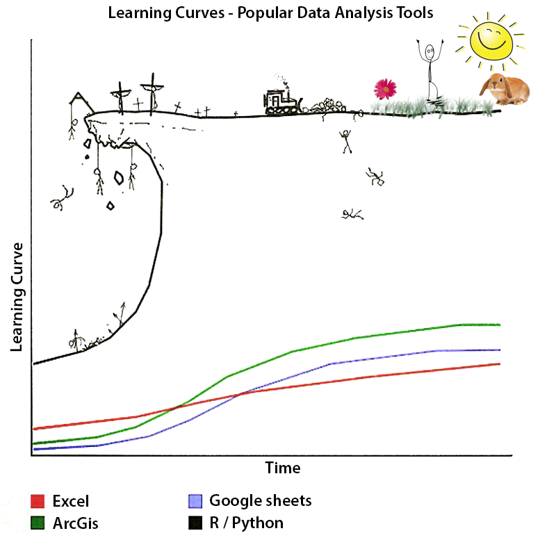
R is not an easy language to learn (see here). At the beginning, the payoff in your investment will not be obvious. You will spend time banging your head on the wall and be tempted to revert to old habits. Having used R for over ten years, I can tell you that the investment is absolutely worth it. Once you’re able to use R, you will have access to an almost endless repository of analytical tools. You will also be more efficient, reproducible, and transparent with your workflows. My advice in the beginning:
- Time spent frustrated is time spent learning. Just because you’re angry doesn’t mean you’re not gaining information.
- Pick something small to begin with. Do not try to port all of your old projects to RStudio, this will come with time.
- Use someone else’s code. It’s often easier to learn a complex problem by seeing someone else’s approach line by line.
- Become a savvy Googler, see the tips above. Hard-copy books are obselete when you have all the information at your finger tips.
- Do not give up!!!
Next time, we’ll talk about data wrangling. This is where the real fun begins…
Attribution
Content in this lesson was pillaged extensively from Jeffrey Hollister (USEPA) and the USGS-R training curriculum here.