Data Wrangling Pt. 2
Lesson Outline
Lesson Exercises
Today’s goals
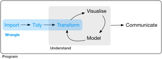
Today we’ll continue our discussion of data wrangling with the tidyverse. Data wrangling is the manipulation or combination of datasets for the purpose of understanding. It fits within the broader scheme of data exploration, described as the art of looking at your data, rapidly generating hypotheses, quickly testing them, then repeating again and again and again (from R for Data Science, as is most of today’s content).
Always remember that wrangling is based on a purpose. The process always begins by answering the following two questions:
- What do my input data look like?
- What should my input data look like given what I want to do?
You define what steps to take to get your data from input to where you want to go.
Last time we learned the following functions from the dplyr package (cheatsheet here):
- Selecting variables with
select - Filtering observations by some criteria with
filter - Adding or modifying existing variables with
mutate - Renaming variables with
rename - Arranging rows by a variable with
arrange
As before, we only have two hours to cover the basics of data wrangling. It’s an unrealistic expectation that you will be a ninja wrangler after this training. As such, the goals are to expose you to fundamentals and to develop an appreciation of what’s possible. I also want to provide resources that you can use for follow-up learning on your own.
Today you should be able to answer (or be able to find answers to) the following:
- How are data joined?
- What is tidy data?
- How do I summarize a dataset?
You should already have the tidyverse and readxl packages installed, but let’s give it a go if you haven’t done this part yet:
# install
install.packages('tidyverse')
After installation, we can load the package:
# load, readxl has to be loaded explicitly
library(tidyverse)
library(readxl)
Exercise 1
As a refresher and to get our brains working, we’re going to repeat the final exercise from our training last week. In this exercise, we’ll make a new project in RStudio and create a script for importing and working with some Bight data today. Alternatively, you can use an existing project from last time.
Create a new project in RStudio or use an existing project from last time. If creating a new project, name it “wrangling_workshop_pt2” or something similar.
Create a new “R Script” in the Source (scripting) Pane, save that file into your project and name it “data_wrangling2.R”.
Add in a comment line at the top stating the purpose. It should look something like:
# Exercise 1: Scripting for data wrangling part 2.Make a folder in your project called
data. You should have downloaded this already, but if not, download the Bight dataset from here: https://github.com/SCCWRP/R_training_2018/raw/master/lessons/data/B13 Chem data.xlsx. Also download some metadata about the Bight stations from here: https://github.com/SCCWRP/R_training_2018/raw/master/lessons/data/Master Data - Station Info.xlsx. Copy these files into thedatafolder in your project.Add some lines to your script to import and store the chemistry data in your Enviroment. The
read_excelfunction from thereadxlpackage is your friend here and the path is"data/B13 Chem data.xlsx". Remember to loadreadxland assign the data to a variable (<-)- Load the
tidyverseand use functions from thedplyrpackage to subset the data. If you can, try to use pipes to link your functions.- Select the columns
StationID,Parameter, andResult - Filter the parameter column to get only
Total_CHLandTotal Organic Carbon(hint: useParameter %in% c('Total_CHL', 'Total Organic Carbon'))
- Select the columns
# import libraries (use install.packages function if not found)
library(tidyverse)
library(readxl)

# import chemistry data, select columns, filter Parameter column
chemdat <- read_excel('data/B13 Chem data.xlsx') %>%
  select(StationID, Parameter, Result) %>%
  filter(Parameter %in% c('Total_CHL', 'Total Organic Carbon'))
Combining data
Combining data is a common task of data wrangling. Perhaps we want to combine information between two datasets that share a common identifier. As a real world example, our Bight data contain information about sediment chemistry and we also want to include metadata about the stations (e.g., depth, lat, lon, etc.). We would need to (and we will) combine data if this information is in two different places. Combining data with dplyr is called joining.
All joins require that each of the tables can be linked by shared identifiers. These are called ‘keys’ and are usually represented as a separate column that acts as a unique variable for the observations. The “Station ID” is a common key, but remember that a key might need to be unique for each row. It doesn’t make sense to join two tables by station ID if multiple site visits were made. In that case, your key should include some information about the site visit and station ID.
Types of joins
The challenge with joins is that the two datasets may not represent the same observations for a given key. For example, you might have one table with all observations for every key, another with only some observations, or two tables with only a few shared keys. What you get back from a join will depend on what’s shared between tables, in addition to the type of join you use.
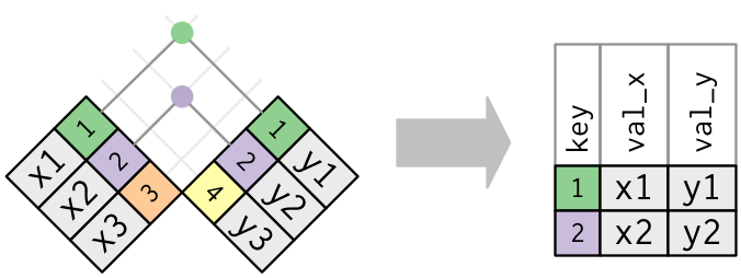
We can demonstrate types of joins with simple graphics. The first is an inner-join.
The second is an outer-join, and comes in three flavors: left, right, and full.
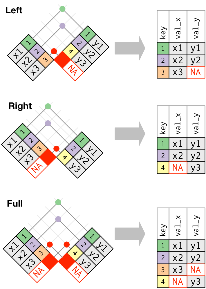
If all keys are shared between two data objects, then left, right, and full joins will give you the same result. I typically only use left_join just because it’s intuitive to me. This assumes that there is never any more information in the second table - it has the same or less keys as the original table.
Remember our mpg dataset?
head(mpg)## manufacturer model displ year cyl trans drv cty hwy fl class
## 1 audi a4 1.8 1999 4 auto(l5) f 18 29 p compact
## 2 audi a4 1.8 1999 4 manual(m5) f 21 29 p compact
## 3 audi a4 2.0 2008 4 manual(m6) f 20 31 p compact
## 4 audi a4 2.0 2008 4 auto(av) f 21 30 p compact
## 5 audi a4 2.8 1999 6 auto(l5) f 16 26 p compact
## 6 audi a4 2.8 1999 6 manual(m5) f 18 26 p compactI’ve made a new data frame (tibble to be specific) of the origin of car manufacturers (domestic, foreign).
# car origin by manufacturer
origin <- tibble(
  manufacturer = c('audi', 'chevrolet', 'dodge', 'ford', 'honda', 'hyundai', 'jeep', 'land rover', 'lincoln', 'mercury', 'nissan', 'pontiac', 'subaru', 'toyota', 'volkswagen'),
  origin = c('for', 'dom', 'dom', 'dom', 'for', 'for', 'dom', 'for', 'dom', 'dom', 'for', 'dom', 'for', 'for', 'for')
)
head(origin)
## # A tibble: 6 x 2
## manufacturer origin
## <chr> <chr>
## 1 audi for
## 2 chevrolet dom
## 3 dodge dom
## 4 ford dom
## 5 honda for
## 6 hyundai forWe want to join this with our mpg dataset.
# join with mpg
mpg <- left_join(mpg, origin, by = 'manufacturer')
head(mpg)
## manufacturer model displ year cyl trans drv cty hwy fl class
## 1 audi a4 1.8 1999 4 auto(l5) f 18 29 p compact
## 2 audi a4 1.8 1999 4 manual(m5) f 21 29 p compact
## 3 audi a4 2.0 2008 4 manual(m6) f 20 31 p compact
## 4 audi a4 2.0 2008 4 auto(av) f 21 30 p compact
## 5 audi a4 2.8 1999 6 auto(l5) f 16 26 p compact
## 6 audi a4 2.8 1999 6 manual(m5) f 18 26 p compact
## origin
## 1 for
## 2 for
## 3 for
## 4 for
## 5 for
## 6 forThere you have it. As a side note, this is also a one-to-many join (i.e., there were many keys in the first table that corresponded to only one key in the second table).
Exercise 2
For this exercise we’ll use two datasets from Bight13. We’re going to use the wrangled dataset we created in exercise 1, import a metadata table with lat/lon, and join the two by StationID. We’ll have to do a bit of wrangling with the metadata.
Make sure you have the wrangled chemistry data in your environment from exercise 1 (check with
ls()or the Environment pane in RStudio). If not, run the code in the answer box above.Import the
Master Data - Station Info.xlsxfile in your data folder withread_excel. Save it as an object in your workspace.Select only the
StationID,StationWaterDepth,SampleLatitude, andSampleLongitudecolumns from the master data.Rename the
StationWaterDepth,SampleLatitude, andSampleLongitudecolumns asdepth,lat, andlon.Use
left_jointo combine the metadata with the chemistry data you created in exercise one. Use theStationIDcolumn as the key. Save it as a new object in your environment.Check the dimensions of the new table. How many rows do we have compared to the original chemistry data? How many columns?
# import metadata, select and rename columns
metadat <- read_excel('data/Master Data - Station Info.xlsx') %>%
  select(StationID, StationWaterDepth, SampleLatitude, SampleLongitude) %>%
  rename(
    depth = StationWaterDepth,
    lat = SampleLatitude,
    lon = SampleLongitude
  )

# dimensions of metadat, chemdat
dim(metadat)
dim(chemdat)

# join chemdat with metadat, check dimensions
alldat <- left_join(chemdat, metadat, by = 'StationID')
dim(alldat)
Tidy data
The opposite of a tidy dataset is a messy dataset. You should always strive to create a tidy data set as an outcome of the wrangling process. Tidy data are easy to work with and will make downstream analysis much simpler. This will become apparent when we start summarizing and plotting our data.
To help understand tidy data, it’s useful to look at alternative ways of representing data. The example below shows the same data organised in four different ways. Each dataset shows the same values of four variables country, year, population, and cases, but each dataset organises the values in a different way. Only one of these examples is tidy.
table1## # A tibble: 6 x 4
## country year cases population
## <chr> <int> <int> <int>
## 1 Afghanistan 1999 745 19987071
## 2 Afghanistan 2000 2666 20595360
## 3 Brazil 1999 37737 172006362
## 4 Brazil 2000 80488 174504898
## 5 China 1999 212258 1272915272
## 6 China 2000 213766 1280428583table2## # A tibble: 12 x 4
## country year type count
## <chr> <int> <chr> <int>
## 1 Afghanistan 1999 cases 745
## 2 Afghanistan 1999 population 19987071
## 3 Afghanistan 2000 cases 2666
## 4 Afghanistan 2000 population 20595360
## 5 Brazil 1999 cases 37737
## 6 Brazil 1999 population 172006362
## 7 Brazil 2000 cases 80488
## 8 Brazil 2000 population 174504898
## 9 China 1999 cases 212258
## 10 China 1999 population 1272915272
## 11 China 2000 cases 213766
## 12 China 2000 population 1280428583table3## # A tibble: 6 x 3
## country year rate
## * <chr> <int> <chr>
## 1 Afghanistan 1999 745/19987071
## 2 Afghanistan 2000 2666/20595360
## 3 Brazil 1999 37737/172006362
## 4 Brazil 2000 80488/174504898
## 5 China 1999 212258/1272915272
## 6 China 2000 213766/1280428583# Spread across two tibbles
table4a # cases## # A tibble: 3 x 3
## country `1999` `2000`
## * <chr> <int> <int>
## 1 Afghanistan 745 2666
## 2 Brazil 37737 80488
## 3 China 212258 213766table4b # population## # A tibble: 3 x 3
## country `1999` `2000`
## * <chr> <int> <int>
## 1 Afghanistan 19987071 20595360
## 2 Brazil 172006362 174504898
## 3 China 1272915272 1280428583These are all representations of the same underlying data but they are not equally easy to work with. The tidy dataset is much easier to work with inside the tidyverse.
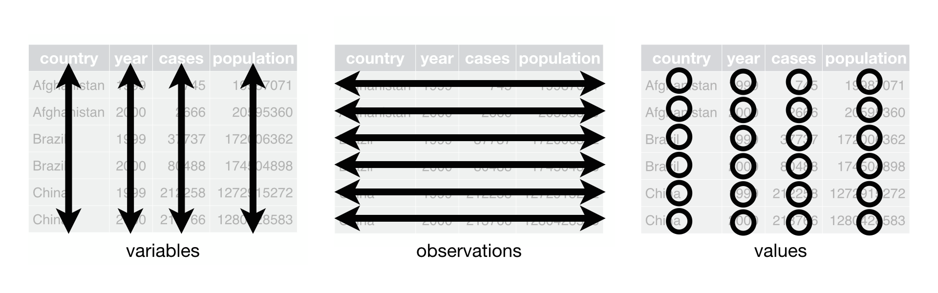
There are three inter-correlated rules which make a dataset tidy:
- Each variable must have its own column.
- Each observation must have its own row.
- Each value must have its own cell.
There are some very real reasons why you would encounter untidy data:
Most people aren’t familiar with the principles of tidy data, and it’s hard to derive them yourself unless you spend a lot of time working with data.
Data is often organised to facilitate some use other than analysis. For example, data is often organised to make entry as easy as possible.
This means for most real analyses, you’ll need to do some tidying. The first step is always to figure out what the variables and observations are. The second step is to resolve one of two common problems:
One variable might be spread across multiple columns.
One observation might be scattered across multiple rows.
To fix these problems, you’ll need the two most important functions in tidyr: gather() and spread().
Gathering
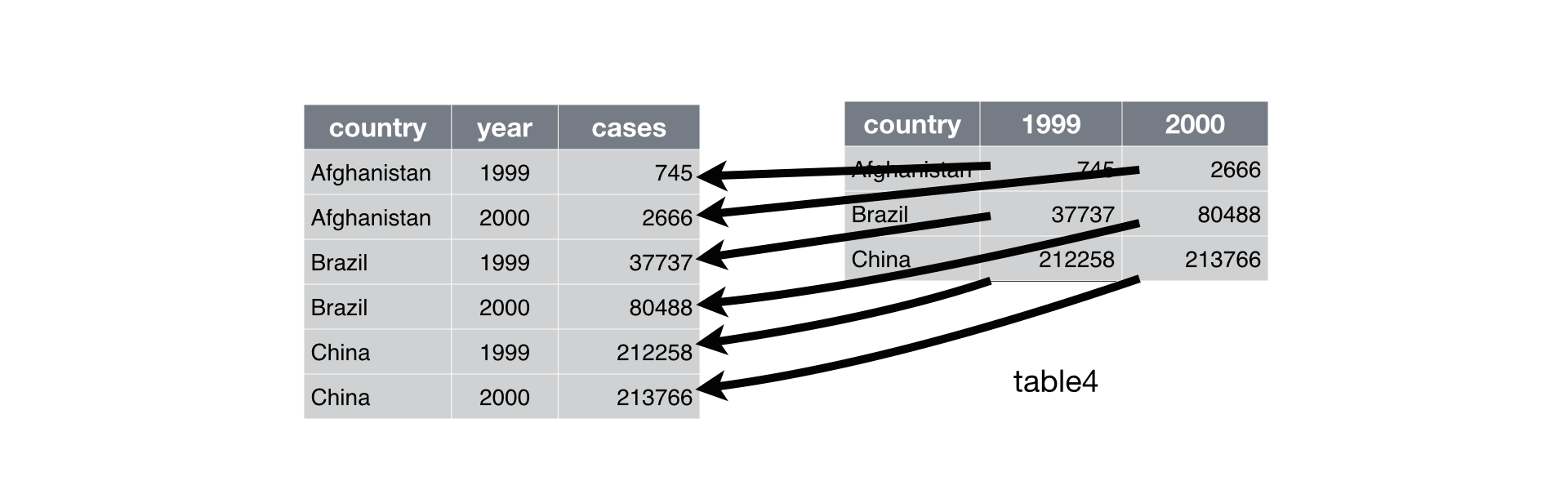
A common problem is a dataset where some of the column names are not names of variables, but values of a variable. Take table4a: the column names 1999 and 2000 represent values of the year variable, and each row represents two observations, not one.
table4a## # A tibble: 3 x 3
## country `1999` `2000`
## * <chr> <int> <int>
## 1 Afghanistan 745 2666
## 2 Brazil 37737 80488
## 3 China 212258 213766To tidy a dataset like this, we need to gather those columns into a new pair of variables. To describe that operation we need three parameters:
The set of columns that represent values, not variables. In this example, those are the columns
1999and2000.The name of the variable whose values form the column names. I call that the
key, and here it isyear.The name of the variable whose values are spread over the cells. I call that
value, and here it’s the number ofcases.
Together those parameters generate the call to gather():
table4a %>%
  gather(`1999`, `2000`, key = "year", value = "cases")
## # A tibble: 6 x 3
## country year cases
## <chr> <chr> <int>
## 1 Afghanistan 1999 745
## 2 Brazil 1999 37737
## 3 China 1999 212258
## 4 Afghanistan 2000 2666
## 5 Brazil 2000 80488
## 6 China 2000 213766Gathering can be graphically demonstrated:
Spreading
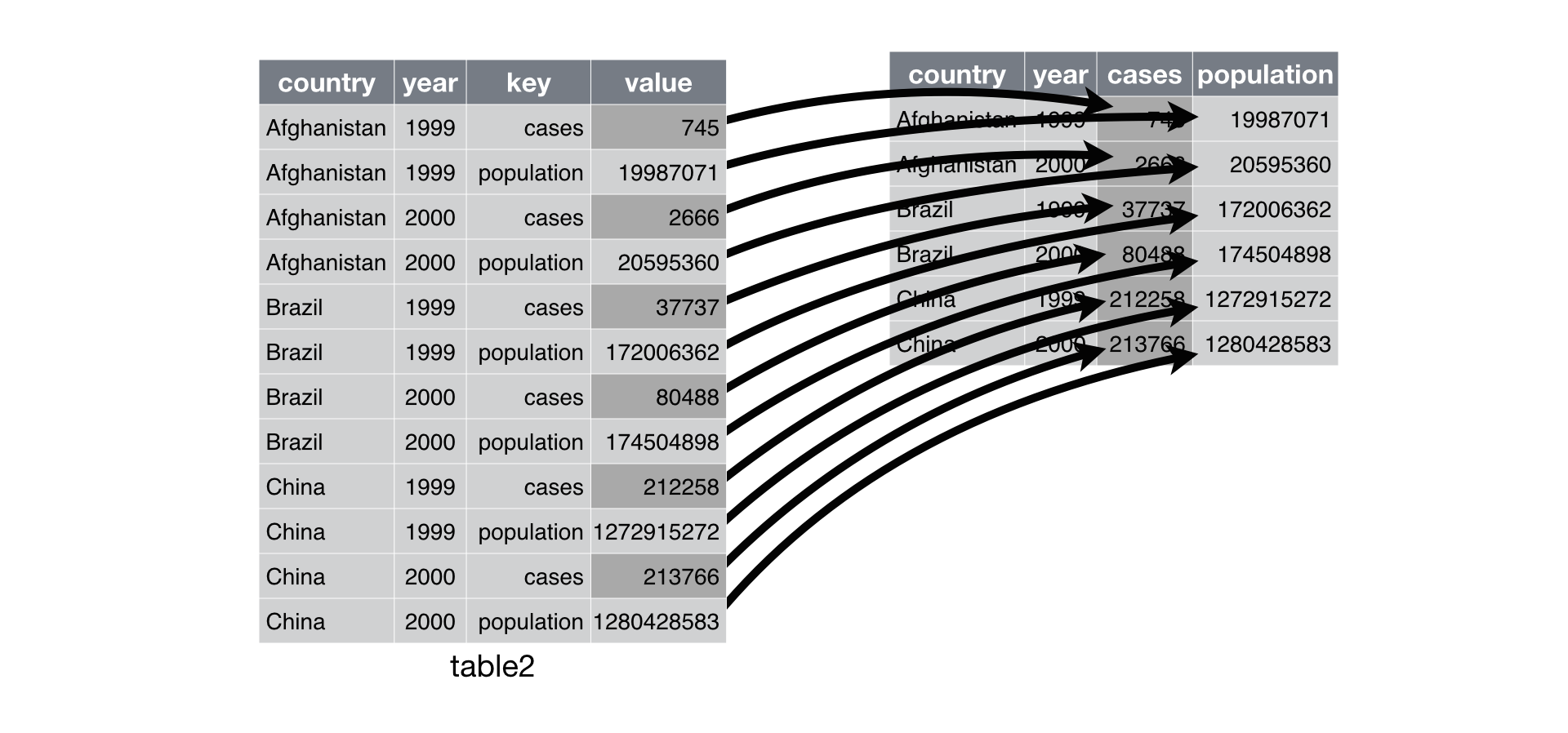
Spreading is the opposite of gathering. You use it when an observation is scattered across multiple rows. For example, take table2: an observation is a country in a year, but each observation is spread across two rows.
table2## # A tibble: 12 x 4
## country year type count
## <chr> <int> <chr> <int>
## 1 Afghanistan 1999 cases 745
## 2 Afghanistan 1999 population 19987071
## 3 Afghanistan 2000 cases 2666
## 4 Afghanistan 2000 population 20595360
## 5 Brazil 1999 cases 37737
## 6 Brazil 1999 population 172006362
## 7 Brazil 2000 cases 80488
## 8 Brazil 2000 population 174504898
## 9 China 1999 cases 212258
## 10 China 1999 population 1272915272
## 11 China 2000 cases 213766
## 12 China 2000 population 1280428583To tidy this up, we first analyse the representation in similar way to gather(). This time, however, we only need two parameters:
The column that contains variable names, the
keycolumn. Here, it’stype.The column that contains values forms multiple variables, the
valuecolumn. Here it’scount.
Once we’ve figured that out, we can use spread(), as shown programmatically below.
spread(table2, key = type, value = count)## # A tibble: 6 x 4
## country year cases population
## <chr> <int> <int> <int>
## 1 Afghanistan 1999 745 19987071
## 2 Afghanistan 2000 2666 20595360
## 3 Brazil 1999 37737 172006362
## 4 Brazil 2000 80488 174504898
## 5 China 1999 212258 1272915272
## 6 China 2000 213766 1280428583Spreading can be graphically demonstrated:
Exercise 3
Let’s take a look at our combined dataset we created in exercise 2. Are these tidy data? What rules do they violate? We can use the functions in the tidyr package from the tidyverse to make these data tidy.
Inspect the combined dataset you created in exercise 2. What are the dimensions (hint:
dim)? What are the names and column types (hint:str)?We need to make these data tidy. Which column is your key? Which column is the value?
Use the
spreadfunction to make the data tidy. Assign the new tidy dataset to a variable in your environment.Check the dimensions and structure of your new dataset. What’s different?
Rename the
Total Organic Carboncolumn toTOC. You can use therenamefunction but you have to enclose the old column name with backticks (the second symbol on the tilde key). Any variable with spaces or non-standard characters can be referenced by enclosing it with backticks (see here).
# check dimensions, structure
dim(alldat)
str(alldat)

# tidy alldat
tidydat <- alldat %>%
  spread(key = 'Parameter', value = 'Result')

# check dimensions, structure
dim(tidydat)
str(tidydat)

# rename to TOC
tidydat <- tidydat %>%
  rename(
    TOC = `Total Organic Carbon`
  )
Group by and summarize
The last tool we’re going to learn about in dplyr is the summarize function. As the name implies, this function lets you summarize columns in a dataset. Think of it as a way to condense rows using a summary method of your choice, e.g., what’s the average of the values in a column?
The summarize function is most useful with the group_by function. This function lets you define a column that serves as a grouping variable for developing separate summaries, as compared to summarizing the entire dataset. The group_by function works with any dplyr function so it can be quite powerful.
Let’s return to our mpg dataset.
head(mpg)## manufacturer model displ year cyl trans drv cty hwy fl class
## 1 audi a4 1.8 1999 4 auto(l5) f 18 29 p compact
## 2 audi a4 1.8 1999 4 manual(m5) f 21 29 p compact
## 3 audi a4 2.0 2008 4 manual(m6) f 20 31 p compact
## 4 audi a4 2.0 2008 4 auto(av) f 21 30 p compact
## 5 audi a4 2.8 1999 6 auto(l5) f 16 26 p compact
## 6 audi a4 2.8 1999 6 manual(m5) f 18 26 p compact
## origin
## 1 for
## 2 for
## 3 for
## 4 for
## 5 for
## 6 forThis is not a terribly interesting dataset until we start to evaluate some of the differences. It’s also setup in a way to let us easily group by different variables. We could ask a simple question: how does highway mileage differ by manufacturer?
First we can use group_by. Notice the new information at the top of the output.
by_make <- group_by(mpg, manufacturer)
by_make
## # A tibble: 234 x 12
## # Groups: manufacturer [15]
## manufacturer model displ year cyl trans drv cty hwy fl
## <chr> <chr> <dbl> <int> <int> <chr> <chr> <int> <int> <chr>
## 1 audi a4 1.80 1999 4 auto(l~ f 18 29 p
## 2 audi a4 1.80 1999 4 manual~ f 21 29 p
## 3 audi a4 2.00 2008 4 manual~ f 20 31 p
## 4 audi a4 2.00 2008 4 auto(a~ f 21 30 p
## 5 audi a4 2.80 1999 6 auto(l~ f 16 26 p
## 6 audi a4 2.80 1999 6 manual~ f 18 26 p
## 7 audi a4 3.10 2008 6 auto(a~ f 18 27 p
## 8 audi a4 quat~ 1.80 1999 4 manual~ 4 18 26 p
## 9 audi a4 quat~ 1.80 1999 4 auto(l~ 4 16 25 p
## 10 audi a4 quat~ 2.00 2008 4 manual~ 4 20 28 p
## # ... with 224 more rows, and 2 more variables: class <chr>, origin <chr>We can then summarize to get the average mileage by group.
by_make <- summarize(by_make, ave_hwy = mean(hwy))
by_make
## # A tibble: 15 x 2
## manufacturer ave_hwy
## <chr> <dbl>
## 1 audi 26.4
## 2 chevrolet 21.9
## 3 dodge 17.9
## 4 ford 19.4
## 5 honda 32.6
## 6 hyundai 26.9
## 7 jeep 17.6
## 8 land rover 16.5
## 9 lincoln 17.0
## 10 mercury 18.0
## 11 nissan 24.6
## 12 pontiac 26.4
## 13 subaru 25.6
## 14 toyota 24.9
## 15 volkswagen 29.2Of course, this can (and should) be done with pipes:
by_make <- mpg %>%
  group_by(manufacturer) %>%
  summarize(ave_hwy = mean(hwy))
by_make
## # A tibble: 15 x 2
## manufacturer ave_hwy
## <chr> <dbl>
## 1 audi 26.4
## 2 chevrolet 21.9
## 3 dodge 17.9
## 4 ford 19.4
## 5 honda 32.6
## 6 hyundai 26.9
## 7 jeep 17.6
## 8 land rover 16.5
## 9 lincoln 17.0
## 10 mercury 18.0
## 11 nissan 24.6
## 12 pontiac 26.4
## 13 subaru 25.6
## 14 toyota 24.9
## 15 volkswagen 29.2We can group the dataset by more than one column to get summaries with multiple groups. Here we can look at mileage by each unique combination of year and drive-train (forward, rear, all)
by_yr_drv <- mpg %>%
  group_by(year, drv) %>%
  summarize(ave_hwy = mean(hwy))
by_yr_drv
## # A tibble: 6 x 3
## # Groups: year [?]
## year drv ave_hwy
## <int> <chr> <dbl>
## 1 1999 4 18.8
## 2 1999 f 27.9
## 3 1999 r 20.6
## 4 2008 4 19.5
## 5 2008 f 28.4
## 6 2008 r 21.3We can also get more than one summary at a time. The summary function can use any function that operates on a vector. Some common examples include min, max, sd, var, median, mean, and n. It’s usually good practice to include a summary of how many observations were in each group, so get used to including the n function.
more_sums <- mpg %>%
  group_by(manufacturer) %>%
  summarize(
    n = n(),
    min_hwy = min(hwy),
    max_hwy = max(hwy),
    ave_hwy = mean(hwy)
  )
more_sums
## # A tibble: 15 x 5
## manufacturer n min_hwy max_hwy ave_hwy
## <chr> <int> <dbl> <dbl> <dbl>
## 1 audi 18 23. 31. 26.4
## 2 chevrolet 19 14. 30. 21.9
## 3 dodge 37 12. 24. 17.9
## 4 ford 25 15. 26. 19.4
## 5 honda 9 29. 36. 32.6
## 6 hyundai 14 24. 31. 26.9
## 7 jeep 8 12. 22. 17.6
## 8 land rover 4 15. 18. 16.5
## 9 lincoln 3 16. 18. 17.0
## 10 mercury 4 17. 19. 18.0
## 11 nissan 13 17. 32. 24.6
## 12 pontiac 5 25. 28. 26.4
## 13 subaru 14 23. 27. 25.6
## 14 toyota 34 15. 37. 24.9
## 15 volkswagen 27 23. 44. 29.2The group_by function can work with both categorical and numeric variables. In most cases, summarizing by a numeric variable will not be very informative because of many unique observations that define a “group”. We can categorize a continuous variable to make the summary more informative. For example, maybe we want to summarize some data based on observations that are “low” or “high” for a continuous variable. We can make a new categorical variable and use the tricks we just learned to summarize by the new grouping.
Let’s look at the displacement variable in the mpg dataset. This is a measure of engine size.
mean(mpg$displ)## [1] 3.471795range(mpg$displ)## [1] 1.6 7.0Maybe we want to summarize mileage for engines that are small or large. Let’s replace the original displacement column with one that categorizes engine size using the average value as the breakpoint.
displ_cat <- mpg %>%
  mutate(
    displ = ifelse(displ < 3.47, 'small', 'large')
  )
displ_cat
## manufacturer model displ year cyl trans drv cty
## 1 audi a4 small 1999 4 auto(l5) f 18
## 2 audi a4 small 1999 4 manual(m5) f 21
## 3 audi a4 small 2008 4 manual(m6) f 20
## 4 audi a4 small 2008 4 auto(av) f 21
## 5 audi a4 small 1999 6 auto(l5) f 16
## 6 audi a4 small 1999 6 manual(m5) f 18
## 7 audi a4 small 2008 6 auto(av) f 18
## 8 audi a4 quattro small 1999 4 manual(m5) 4 18
## 9 audi a4 quattro small 1999 4 auto(l5) 4 16
## 10 audi a4 quattro small 2008 4 manual(m6) 4 20
## 11 audi a4 quattro small 2008 4 auto(s6) 4 19
## 12 audi a4 quattro small 1999 6 auto(l5) 4 15
## 13 audi a4 quattro small 1999 6 manual(m5) 4 17
## 14 audi a4 quattro small 2008 6 auto(s6) 4 17
## 15 audi a4 quattro small 2008 6 manual(m6) 4 15
## 16 audi a6 quattro small 1999 6 auto(l5) 4 15
## 17 audi a6 quattro small 2008 6 auto(s6) 4 17
## 18 audi a6 quattro large 2008 8 auto(s6) 4 16
## 19 chevrolet c1500 suburban 2wd large 2008 8 auto(l4) r 14
## 20 chevrolet c1500 suburban 2wd large 2008 8 auto(l4) r 11
## 21 chevrolet c1500 suburban 2wd large 2008 8 auto(l4) r 14
## 22 chevrolet c1500 suburban 2wd large 1999 8 auto(l4) r 13
## 23 chevrolet c1500 suburban 2wd large 2008 8 auto(l4) r 12
## 24 chevrolet corvette large 1999 8 manual(m6) r 16
## 25 chevrolet corvette large 1999 8 auto(l4) r 15
## 26 chevrolet corvette large 2008 8 manual(m6) r 16
## 27 chevrolet corvette large 2008 8 auto(s6) r 15
## 28 chevrolet corvette large 2008 8 manual(m6) r 15
## 29 chevrolet k1500 tahoe 4wd large 2008 8 auto(l4) 4 14
## 30 chevrolet k1500 tahoe 4wd large 2008 8 auto(l4) 4 11
## 31 chevrolet k1500 tahoe 4wd large 1999 8 auto(l4) 4 11
## 32 chevrolet k1500 tahoe 4wd large 1999 8 auto(l4) 4 14
## 33 chevrolet malibu small 1999 4 auto(l4) f 19
## 34 chevrolet malibu small 2008 4 auto(l4) f 22
## 35 chevrolet malibu small 1999 6 auto(l4) f 18
## 36 chevrolet malibu large 2008 6 auto(l4) f 18
## 37 chevrolet malibu large 2008 6 auto(s6) f 17
## 38 dodge caravan 2wd small 1999 4 auto(l3) f 18
## 39 dodge caravan 2wd small 1999 6 auto(l4) f 17
## 40 dodge caravan 2wd small 1999 6 auto(l4) f 16
## 41 dodge caravan 2wd small 1999 6 auto(l4) f 16
## 42 dodge caravan 2wd small 2008 6 auto(l4) f 17
## 43 dodge caravan 2wd small 2008 6 auto(l4) f 17
## 44 dodge caravan 2wd small 2008 6 auto(l4) f 11
## 45 dodge caravan 2wd large 1999 6 auto(l4) f 15
## 46 dodge caravan 2wd large 1999 6 auto(l4) f 15
## 47 dodge caravan 2wd large 2008 6 auto(l6) f 16
## 48 dodge caravan 2wd large 2008 6 auto(l6) f 16
## 49 dodge dakota pickup 4wd large 2008 6 manual(m6) 4 15
## 50 dodge dakota pickup 4wd large 2008 6 auto(l4) 4 14
## 51 dodge dakota pickup 4wd large 1999 6 auto(l4) 4 13
## 52 dodge dakota pickup 4wd large 1999 6 manual(m5) 4 14
## 53 dodge dakota pickup 4wd large 2008 8 auto(l5) 4 14
## 54 dodge dakota pickup 4wd large 2008 8 auto(l5) 4 14
## 55 dodge dakota pickup 4wd large 2008 8 auto(l5) 4 9
## 56 dodge dakota pickup 4wd large 1999 8 manual(m5) 4 11
## 57 dodge dakota pickup 4wd large 1999 8 auto(l4) 4 11
## 58 dodge durango 4wd large 1999 6 auto(l4) 4 13
## 59 dodge durango 4wd large 2008 8 auto(l5) 4 13
## 60 dodge durango 4wd large 2008 8 auto(l5) 4 9
## 61 dodge durango 4wd large 2008 8 auto(l5) 4 13
## 62 dodge durango 4wd large 1999 8 auto(l4) 4 11
## 63 dodge durango 4wd large 2008 8 auto(l5) 4 13
## 64 dodge durango 4wd large 1999 8 auto(l4) 4 11
## 65 dodge ram 1500 pickup 4wd large 2008 8 manual(m6) 4 12
## 66 dodge ram 1500 pickup 4wd large 2008 8 auto(l5) 4 9
## 67 dodge ram 1500 pickup 4wd large 2008 8 auto(l5) 4 13
## 68 dodge ram 1500 pickup 4wd large 2008 8 auto(l5) 4 13
## 69 dodge ram 1500 pickup 4wd large 2008 8 manual(m6) 4 12
## 70 dodge ram 1500 pickup 4wd large 2008 8 manual(m6) 4 9
## 71 dodge ram 1500 pickup 4wd large 1999 8 auto(l4) 4 11
## 72 dodge ram 1500 pickup 4wd large 1999 8 manual(m5) 4 11
## 73 dodge ram 1500 pickup 4wd large 2008 8 auto(l5) 4 13
## 74 dodge ram 1500 pickup 4wd large 1999 8 auto(l4) 4 11
## 75 ford expedition 2wd large 1999 8 auto(l4) r 11
## 76 ford expedition 2wd large 1999 8 auto(l4) r 11
## 77 ford expedition 2wd large 2008 8 auto(l6) r 12
## 78 ford explorer 4wd large 1999 6 auto(l5) 4 14
## 79 ford explorer 4wd large 1999 6 manual(m5) 4 15
## 80 ford explorer 4wd large 1999 6 auto(l5) 4 14
## 81 ford explorer 4wd large 2008 6 auto(l5) 4 13
## 82 ford explorer 4wd large 2008 8 auto(l6) 4 13
## 83 ford explorer 4wd large 1999 8 auto(l4) 4 13
## 84 ford f150 pickup 4wd large 1999 6 auto(l4) 4 14
## 85 ford f150 pickup 4wd large 1999 6 manual(m5) 4 14
## 86 ford f150 pickup 4wd large 1999 8 manual(m5) 4 13
## 87 ford f150 pickup 4wd large 1999 8 auto(l4) 4 13
## 88 ford f150 pickup 4wd large 2008 8 auto(l4) 4 13
## 89 ford f150 pickup 4wd large 1999 8 auto(l4) 4 11
## 90 ford f150 pickup 4wd large 2008 8 auto(l4) 4 13
## 91 ford mustang large 1999 6 manual(m5) r 18
## 92 ford mustang large 1999 6 auto(l4) r 18
## 93 ford mustang large 2008 6 manual(m5) r 17
## 94 ford mustang large 2008 6 auto(l5) r 16
## 95 ford mustang large 1999 8 auto(l4) r 15
## 96 ford mustang large 1999 8 manual(m5) r 15
## 97 ford mustang large 2008 8 manual(m5) r 15
## 98 ford mustang large 2008 8 auto(l5) r 15
## 99 ford mustang large 2008 8 manual(m6) r 14
## 100 honda civic small 1999 4 manual(m5) f 28
## 101 honda civic small 1999 4 auto(l4) f 24
## 102 honda civic small 1999 4 manual(m5) f 25
## 103 honda civic small 1999 4 manual(m5) f 23
## 104 honda civic small 1999 4 auto(l4) f 24
## 105 honda civic small 2008 4 manual(m5) f 26
## 106 honda civic small 2008 4 auto(l5) f 25
## 107 honda civic small 2008 4 auto(l5) f 24
## 108 honda civic small 2008 4 manual(m6) f 21
## 109 hyundai sonata small 1999 4 auto(l4) f 18
## 110 hyundai sonata small 1999 4 manual(m5) f 18
## 111 hyundai sonata small 2008 4 auto(l4) f 21
## 112 hyundai sonata small 2008 4 manual(m5) f 21
## 113 hyundai sonata small 1999 6 auto(l4) f 18
## 114 hyundai sonata small 1999 6 manual(m5) f 18
## 115 hyundai sonata small 2008 6 auto(l5) f 19
## 116 hyundai tiburon small 1999 4 auto(l4) f 19
## 117 hyundai tiburon small 1999 4 manual(m5) f 19
## 118 hyundai tiburon small 2008 4 manual(m5) f 20
## 119 hyundai tiburon small 2008 4 auto(l4) f 20
## 120 hyundai tiburon small 2008 6 auto(l4) f 17
## 121 hyundai tiburon small 2008 6 manual(m6) f 16
## 122 hyundai tiburon small 2008 6 manual(m5) f 17
## 123 jeep grand cherokee 4wd small 2008 6 auto(l5) 4 17
## 124 jeep grand cherokee 4wd large 2008 6 auto(l5) 4 15
## 125 jeep grand cherokee 4wd large 1999 6 auto(l4) 4 15
## 126 jeep grand cherokee 4wd large 1999 8 auto(l4) 4 14
## 127 jeep grand cherokee 4wd large 2008 8 auto(l5) 4 9
## 128 jeep grand cherokee 4wd large 2008 8 auto(l5) 4 14
## 129 jeep grand cherokee 4wd large 2008 8 auto(l5) 4 13
## 130 jeep grand cherokee 4wd large 2008 8 auto(l5) 4 11
## 131 land rover range rover large 1999 8 auto(l4) 4 11
## 132 land rover range rover large 2008 8 auto(s6) 4 12
## 133 land rover range rover large 2008 8 auto(s6) 4 12
## 134 land rover range rover large 1999 8 auto(l4) 4 11
## 135 lincoln navigator 2wd large 1999 8 auto(l4) r 11
## 136 lincoln navigator 2wd large 1999 8 auto(l4) r 11
## 137 lincoln navigator 2wd large 2008 8 auto(l6) r 12
## 138 mercury mountaineer 4wd large 1999 6 auto(l5) 4 14
## 139 mercury mountaineer 4wd large 2008 6 auto(l5) 4 13
## 140 mercury mountaineer 4wd large 2008 8 auto(l6) 4 13
## 141 mercury mountaineer 4wd large 1999 8 auto(l4) 4 13
## 142 nissan altima small 1999 4 manual(m5) f 21
## 143 nissan altima small 1999 4 auto(l4) f 19
## 144 nissan altima small 2008 4 auto(av) f 23
## 145 nissan altima small 2008 4 manual(m6) f 23
## 146 nissan altima large 2008 6 manual(m6) f 19
## 147 nissan altima large 2008 6 auto(av) f 19
## 148 nissan maxima small 1999 6 auto(l4) f 18
## 149 nissan maxima small 1999 6 manual(m5) f 19
## 150 nissan maxima large 2008 6 auto(av) f 19
## 151 nissan pathfinder 4wd small 1999 6 auto(l4) 4 14
## 152 nissan pathfinder 4wd small 1999 6 manual(m5) 4 15
## 153 nissan pathfinder 4wd large 2008 6 auto(l5) 4 14
## 154 nissan pathfinder 4wd large 2008 8 auto(s5) 4 12
## 155 pontiac grand prix small 1999 6 auto(l4) f 18
## 156 pontiac grand prix large 1999 6 auto(l4) f 16
## 157 pontiac grand prix large 1999 6 auto(l4) f 17
## 158 pontiac grand prix large 2008 6 auto(l4) f 18
## 159 pontiac grand prix large 2008 8 auto(s4) f 16
## 160 subaru forester awd small 1999 4 manual(m5) 4 18
## 161 subaru forester awd small 1999 4 auto(l4) 4 18
## 162 subaru forester awd small 2008 4 manual(m5) 4 20
## 163 subaru forester awd small 2008 4 manual(m5) 4 19
## 164 subaru forester awd small 2008 4 auto(l4) 4 20
## 165 subaru forester awd small 2008 4 auto(l4) 4 18
## 166 subaru impreza awd small 1999 4 auto(l4) 4 21
## 167 subaru impreza awd small 1999 4 manual(m5) 4 19
## 168 subaru impreza awd small 1999 4 manual(m5) 4 19
## 169 subaru impreza awd small 1999 4 auto(l4) 4 19
## 170 subaru impreza awd small 2008 4 auto(s4) 4 20
## 171 subaru impreza awd small 2008 4 auto(s4) 4 20
## 172 subaru impreza awd small 2008 4 manual(m5) 4 19
## 173 subaru impreza awd small 2008 4 manual(m5) 4 20
## 174 toyota 4runner 4wd small 1999 4 manual(m5) 4 15
## 175 toyota 4runner 4wd small 1999 4 auto(l4) 4 16
## 176 toyota 4runner 4wd small 1999 6 auto(l4) 4 15
## 177 toyota 4runner 4wd small 1999 6 manual(m5) 4 15
## 178 toyota 4runner 4wd large 2008 6 auto(l5) 4 16
## 179 toyota 4runner 4wd large 2008 8 auto(l5) 4 14
## 180 toyota camry small 1999 4 manual(m5) f 21
## 181 toyota camry small 1999 4 auto(l4) f 21
## 182 toyota camry small 2008 4 manual(m5) f 21
## 183 toyota camry small 2008 4 auto(l5) f 21
## 184 toyota camry small 1999 6 auto(l4) f 18
## 185 toyota camry small 1999 6 manual(m5) f 18
## 186 toyota camry large 2008 6 auto(s6) f 19
## 187 toyota camry solara small 1999 4 auto(l4) f 21
## 188 toyota camry solara small 1999 4 manual(m5) f 21
## 189 toyota camry solara small 2008 4 manual(m5) f 21
## 190 toyota camry solara small 2008 4 auto(s5) f 22
## 191 toyota camry solara small 1999 6 auto(l4) f 18
## 192 toyota camry solara small 1999 6 manual(m5) f 18
## 193 toyota camry solara small 2008 6 auto(s5) f 18
## 194 toyota corolla small 1999 4 auto(l3) f 24
## 195 toyota corolla small 1999 4 auto(l4) f 24
## 196 toyota corolla small 1999 4 manual(m5) f 26
## 197 toyota corolla small 2008 4 manual(m5) f 28
## 198 toyota corolla small 2008 4 auto(l4) f 26
## 199 toyota land cruiser wagon 4wd large 1999 8 auto(l4) 4 11
## 200 toyota land cruiser wagon 4wd large 2008 8 auto(s6) 4 13
## 201 toyota toyota tacoma 4wd small 1999 4 manual(m5) 4 15
## 202 toyota toyota tacoma 4wd small 1999 4 auto(l4) 4 16
## 203 toyota toyota tacoma 4wd small 2008 4 manual(m5) 4 17
## 204 toyota toyota tacoma 4wd small 1999 6 manual(m5) 4 15
## 205 toyota toyota tacoma 4wd small 1999 6 auto(l4) 4 15
## 206 toyota toyota tacoma 4wd large 2008 6 manual(m6) 4 15
## 207 toyota toyota tacoma 4wd large 2008 6 auto(l5) 4 16
## 208 volkswagen gti small 1999 4 manual(m5) f 21
## 209 volkswagen gti small 1999 4 auto(l4) f 19
## 210 volkswagen gti small 2008 4 manual(m6) f 21
## 211 volkswagen gti small 2008 4 auto(s6) f 22
## 212 volkswagen gti small 1999 6 manual(m5) f 17
## 213 volkswagen jetta small 1999 4 manual(m5) f 33
## 214 volkswagen jetta small 1999 4 manual(m5) f 21
## 215 volkswagen jetta small 1999 4 auto(l4) f 19
## 216 volkswagen jetta small 2008 4 auto(s6) f 22
## 217 volkswagen jetta small 2008 4 manual(m6) f 21
## 218 volkswagen jetta small 2008 5 auto(s6) f 21
## 219 volkswagen jetta small 2008 5 manual(m5) f 21
## 220 volkswagen jetta small 1999 6 auto(l4) f 16
## 221 volkswagen jetta small 1999 6 manual(m5) f 17
## 222 volkswagen new beetle small 1999 4 manual(m5) f 35
## 223 volkswagen new beetle small 1999 4 auto(l4) f 29
## 224 volkswagen new beetle small 1999 4 manual(m5) f 21
## 225 volkswagen new beetle small 1999 4 auto(l4) f 19
## 226 volkswagen new beetle small 2008 5 manual(m5) f 20
## 227 volkswagen new beetle small 2008 5 auto(s6) f 20
## 228 volkswagen passat small 1999 4 manual(m5) f 21
## 229 volkswagen passat small 1999 4 auto(l5) f 18
## 230 volkswagen passat small 2008 4 auto(s6) f 19
## 231 volkswagen passat small 2008 4 manual(m6) f 21
## 232 volkswagen passat small 1999 6 auto(l5) f 16
## 233 volkswagen passat small 1999 6 manual(m5) f 18
## 234 volkswagen passat large 2008 6 auto(s6) f 17
## hwy fl class origin
## 1 29 p compact for
## 2 29 p compact for
## 3 31 p compact for
## 4 30 p compact for
## 5 26 p compact for
## 6 26 p compact for
## 7 27 p compact for
## 8 26 p compact for
## 9 25 p compact for
## 10 28 p compact for
## 11 27 p compact for
## 12 25 p compact for
## 13 25 p compact for
## 14 25 p compact for
## 15 25 p compact for
## 16 24 p midsize for
## 17 25 p midsize for
## 18 23 p midsize for
## 19 20 r suv dom
## 20 15 e suv dom
## 21 20 r suv dom
## 22 17 r suv dom
## 23 17 r suv dom
## 24 26 p 2seater dom
## 25 23 p 2seater dom
## 26 26 p 2seater dom
## 27 25 p 2seater dom
## 28 24 p 2seater dom
## 29 19 r suv dom
## 30 14 e suv dom
## 31 15 r suv dom
## 32 17 d suv dom
## 33 27 r midsize dom
## 34 30 r midsize dom
## 35 26 r midsize dom
## 36 29 r midsize dom
## 37 26 r midsize dom
## 38 24 r minivan dom
## 39 24 r minivan dom
## 40 22 r minivan dom
## 41 22 r minivan dom
## 42 24 r minivan dom
## 43 24 r minivan dom
## 44 17 e minivan dom
## 45 22 r minivan dom
## 46 21 r minivan dom
## 47 23 r minivan dom
## 48 23 r minivan dom
## 49 19 r pickup dom
## 50 18 r pickup dom
## 51 17 r pickup dom
## 52 17 r pickup dom
## 53 19 r pickup dom
## 54 19 r pickup dom
## 55 12 e pickup dom
## 56 17 r pickup dom
## 57 15 r pickup dom
## 58 17 r suv dom
## 59 17 r suv dom
## 60 12 e suv dom
## 61 17 r suv dom
## 62 16 r suv dom
## 63 18 r suv dom
## 64 15 r suv dom
## 65 16 r pickup dom
## 66 12 e pickup dom
## 67 17 r pickup dom
## 68 17 r pickup dom
## 69 16 r pickup dom
## 70 12 e pickup dom
## 71 15 r pickup dom
## 72 16 r pickup dom
## 73 17 r pickup dom
## 74 15 r pickup dom
## 75 17 r suv dom
## 76 17 r suv dom
## 77 18 r suv dom
## 78 17 r suv dom
## 79 19 r suv dom
## 80 17 r suv dom
## 81 19 r suv dom
## 82 19 r suv dom
## 83 17 r suv dom
## 84 17 r pickup dom
## 85 17 r pickup dom
## 86 16 r pickup dom
## 87 16 r pickup dom
## 88 17 r pickup dom
## 89 15 r pickup dom
## 90 17 r pickup dom
## 91 26 r subcompact dom
## 92 25 r subcompact dom
## 93 26 r subcompact dom
## 94 24 r subcompact dom
## 95 21 r subcompact dom
## 96 22 r subcompact dom
## 97 23 r subcompact dom
## 98 22 r subcompact dom
## 99 20 p subcompact dom
## 100 33 r subcompact for
## 101 32 r subcompact for
## 102 32 r subcompact for
## 103 29 p subcompact for
## 104 32 r subcompact for
## 105 34 r subcompact for
## 106 36 r subcompact for
## 107 36 c subcompact for
## 108 29 p subcompact for
## 109 26 r midsize for
## 110 27 r midsize for
## 111 30 r midsize for
## 112 31 r midsize for
## 113 26 r midsize for
## 114 26 r midsize for
## 115 28 r midsize for
## 116 26 r subcompact for
## 117 29 r subcompact for
## 118 28 r subcompact for
## 119 27 r subcompact for
## 120 24 r subcompact for
## 121 24 r subcompact for
## 122 24 r subcompact for
## 123 22 d suv dom
## 124 19 r suv dom
## 125 20 r suv dom
## 126 17 r suv dom
## 127 12 e suv dom
## 128 19 r suv dom
## 129 18 r suv dom
## 130 14 p suv dom
## 131 15 p suv for
## 132 18 r suv for
## 133 18 r suv for
## 134 15 p suv for
## 135 17 r suv dom
## 136 16 p suv dom
## 137 18 r suv dom
## 138 17 r suv dom
## 139 19 r suv dom
## 140 19 r suv dom
## 141 17 r suv dom
## 142 29 r compact for
## 143 27 r compact for
## 144 31 r midsize for
## 145 32 r midsize for
## 146 27 p midsize for
## 147 26 p midsize for
## 148 26 r midsize for
## 149 25 r midsize for
## 150 25 p midsize for
## 151 17 r suv for
## 152 17 r suv for
## 153 20 p suv for
## 154 18 p suv for
## 155 26 r midsize dom
## 156 26 p midsize dom
## 157 27 r midsize dom
## 158 28 r midsize dom
## 159 25 p midsize dom
## 160 25 r suv for
## 161 24 r suv for
## 162 27 r suv for
## 163 25 p suv for
## 164 26 r suv for
## 165 23 p suv for
## 166 26 r subcompact for
## 167 26 r subcompact for
## 168 26 r subcompact for
## 169 26 r subcompact for
## 170 25 p compact for
## 171 27 r compact for
## 172 25 p compact for
## 173 27 r compact for
## 174 20 r suv for
## 175 20 r suv for
## 176 19 r suv for
## 177 17 r suv for
## 178 20 r suv for
## 179 17 r suv for
## 180 29 r midsize for
## 181 27 r midsize for
## 182 31 r midsize for
## 183 31 r midsize for
## 184 26 r midsize for
## 185 26 r midsize for
## 186 28 r midsize for
## 187 27 r compact for
## 188 29 r compact for
## 189 31 r compact for
## 190 31 r compact for
## 191 26 r compact for
## 192 26 r compact for
## 193 27 r compact for
## 194 30 r compact for
## 195 33 r compact for
## 196 35 r compact for
## 197 37 r compact for
## 198 35 r compact for
## 199 15 r suv for
## 200 18 r suv for
## 201 20 r pickup for
## 202 20 r pickup for
## 203 22 r pickup for
## 204 17 r pickup for
## 205 19 r pickup for
## 206 18 r pickup for
## 207 20 r pickup for
## 208 29 r compact for
## 209 26 r compact for
## 210 29 p compact for
## 211 29 p compact for
## 212 24 r compact for
## 213 44 d compact for
## 214 29 r compact for
## 215 26 r compact for
## 216 29 p compact for
## 217 29 p compact for
## 218 29 r compact for
## 219 29 r compact for
## 220 23 r compact for
## 221 24 r compact for
## 222 44 d subcompact for
## 223 41 d subcompact for
## 224 29 r subcompact for
## 225 26 r subcompact for
## 226 28 r subcompact for
## 227 29 r subcompact for
## 228 29 p midsize for
## 229 29 p midsize for
## 230 28 p midsize for
## 231 29 p midsize for
## 232 26 p midsize for
## 233 26 p midsize for
## 234 26 p midsize forNow we can group and summarize.
displ_cat <- displ_cat %>%
  group_by(displ) %>%
  summarize(
    n = n(),
    sd_hwy = sd(hwy),
    ave_hwy = mean(hwy)
  )
displ_cat
## # A tibble: 2 x 4
## displ n sd_hwy ave_hwy
## <chr> <int> <dbl> <dbl>
## 1 large 107 4.04 19.1
## 2 small 127 4.67 27.1The ifelse function works fine for a simple case but what if we want to create more than two categories? You can accomplish this with repeated ifelse statements but this gets messy. For multiple categories, you can use the cut function from base R.
The two important arguments in cut are the breaks and labels that define the cut points and the respective labels for the groups. The labels should always have one less value than breaks. For example, cutting a numeric vector at two points requires four values: absolute minimum, cut point one, cut point two, and absolute maximum. This ensures that the breaks completely describe three groups.
Let’s cut the displacement column into three groups for small, medium, and large engines. The cut points are up to us but for this example we’ll use the 33rd and 66th percentile.
quantile(mpg$displ, probs = c(0.33, 0.66))## 33% 66%
## 2.5 4.0We’ll use cut with the quantiles above (with min/max bounds) and summarize highway mileage by the new groups.
displ_cat <- mpg %>%
  mutate(
    displ = cut(displ, breaks = c(-Inf, 2.5, 4, Inf), labels = c('small', 'medium', 'large'))
    ) %>%
  group_by(displ) %>%
  summarize(
    n = n(),
    std_hwy = sd(hwy),
    ave_hwy = mean(hwy)
  )
displ_cat
## # A tibble: 3 x 4
## displ n std_hwy ave_hwy
## <fct> <int> <dbl> <dbl>
## 1 small 82 3.97 29.2
## 2 medium 81 3.64 22.6
## 3 large 71 3.23 17.6Finally, many of the summary functions we’ve used (e.g., mean, quantile, sd) will not work correctly if there are missing observations in your data. You’ll see these as NA (or sometimes NaN) entries. You have to use the argument na.rm = T to explicitly tell R how to handle the missing values.
x <- c(1, 2, NA, 4)
mean(x)
## [1] NAmean(x, na.rm = T)## [1] 2.333333A quick check for missing values can be done with anyNA. This works on vectors and data frames.
anyNA(x)## [1] TRUEExercise 4
Now we have access to a several tools in the tidyverse to help us wrangle more effectively. For the final exercise, we’re going to get some summary data on our Bight dataset. We’re going to summarize by depth, which will require us to create a categorical variable. Once this is done we’ll see how chlorophyll varies with shallow and deep depths. Don’t forget that you’ll have to use the optional argument na.rm = T if you have missing values (hint anyNA(tidydat$Total_CHL) to check).
Using the tidy data we created in exercise 3, take a look at the range of values in the depth column (hint
range(tidydat$depth)or look at quantiles withquantile).Pick some cut points for the depth column to define the difference between shallow and deep depths. Use the
cutfunction withmutateto create a new categorical column for depth. Call this new columndepth_cat(hint:newdat <- mutate(newdat, depth_cat = cut(...)))Group the dataset by the new depth variable using
group_by.Get some summaries of chlorophyll using
summarize. Try to get the number of samples, average, median, and variance of observations (hint:n,mean,median,var). Don’t forget to usena.rm = Tif there are missing observations. Did you get the summaries you wanted?Repeat the exercise but create more categories for depth (e.g., shallow, mid, deep). Do you still see the same patterns?
sumdat <- tidydat %>%
  mutate(
    depth_cat = cut(depth, breaks = c(-Inf, 15, 150, Inf), labels = c('shallow', 'mid', 'deep'))
  ) %>%
  group_by(depth_cat) %>%
  summarize(
    n = n(),
    ave_chl = mean(Total_CHL, na.rm = T),
    med_chl = median(Total_CHL, na.rm = T),
    var_chl = var(Total_CHL, na.rm = T)
  )
sumdat
Next time
Now you should be able to answer (or be able to find answers to) the following:
- How are data joined?
- What is tidy data?
- How do I summarize a dataset?
Next time we’ll learn about data visualization and graphics.
Attribution
Content in this lesson was pillaged extensively from the USGS-R training curriculum here and R for data Science.