Data Wrangling Pt. 1
Lesson Outline
Lesson Exercises
Today’s goals
Data wrangling (manipulation, ninjery, cleaning, etc.) is the part of any data analysis that will take the most time. While it may not necessarily be fun, it is foundational to all the work that follows. I strongly believe that mastering these skills has more value than mastering a particular analysis. Check out this article if you don’t believe me.
As before, we only have two hours to cover the basics of data wrangling. It’s an unrealistic expectation that you will be a ninja wrangler after this training. As such, the goals are to expose you to fundamentals and to develop an appreciation of what’s possible. I also want to provide resources that you can use for follow-up learning on your own.
Today you should be able to answer (or be able to find answers to) the following:
- Why do we need to manipulate data?
- What is the tidyverse?
- What can you do with dplyr?
- What is piping?
Exercise 1
As a refresher and to get our brains working, we’re going to repeat the exercises from our training last week. The only exception is that we’ll be using some data from the Bight. In this exercise, we’ll make a new project in RStudio and create a script for importing and working with these data today.
Start RStudio: To start both R and RStudio requires only firing up RStudio. RStudio should be available from All Programs at the Start Menu. Fire up RStudio. Take a minute or two to orient yourself to the different panes if you need a refresher from last time.
Create a new project. Name it “wrangling_workshop” or something similar.
Create a new “R Script” in the Source (scripting) Pane, save that file into your project and name it “data_wrangling1.R”. It’ll just be a blank text file at this point.
Add in a comment line at the top stating the purpose. It should look something like:
# Exercise 1: Scripting for data wrangling part 1.Make a folder in your project called
data. You should have downloaded this already, but if not, download the Bight dataset from here: https://github.com/SCCWRP/R_training_2018/raw/master/lessons/data/B13 Chem data.xlsx. Also download some metadata about the Bight stations from here: https://github.com/SCCWRP/R_training_2018/raw/master/lessons/data/Master Data - Station Info.xlsx. Copy these files into thedatafolder in your project.Add some lines to your script to import and store the data in your Enviroment. Remember that the data should be in your
datafolder in your project. Theread_excelfunction from thereadxlpackage is your friend here and the paths are"data/B13 Chem data.xlsx"and"data/Master Data - Station Info.xlsx". Remember to install/load thereadxllibrary and to assign the data to a variable (<-)Now run your script and make sure it doesn’t throw any errors and you do in fact get a data frame (or tibble).
Explore the data frame using some of the functions we covered last time (e.g.
head(),dim(), orstr()). This part does not need to be included in the script and can be done directly in the console. It is just a quick QA step to be sure the data read in as expected.
The tidyverse
The tidyverse is a set of packages that work in harmony because they share common data representations and design. The tidyverse package is designed to make it easy to install and load core packages from the tidyverse in a single command. With tidyverse, you’ll be able to address all steps of data exploration.
From the excellent book, R for Data Science, data exploration is the art of looking at your data, rapidly generating hypotheses, quickly testing them, then repeating again and again and again. Tools in the tidyverse also have direct application to more formal analyses with many of the other available R packages on CRAN.
You should already have the tidyverse installed, but let’s give it a go if you haven’t done this part yet:
# install
install.packages('tidyverse')
After installation, we can load the package:
# load
library(tidyverse)
## -- Attaching packages --------------------------------- tidyverse 1.2.1 --## v ggplot2 3.0.0 v readr 1.1.1
## v tibble 1.4.2 v purrr 0.2.5
## v tidyr 0.8.1 v stringr 1.3.1
## v ggplot2 3.0.0 v forcats 0.2.0## -- Conflicts ------------------------------------ tidyverse_conflicts() --
## x dplyr::filter() masks stats::filter()
## x dplyr::lag() masks stats::lag()Notice that the messages you get after loading are a bit different from other packages. That’s because tidyverse is a package that manages other packages. Loading tidyverse will load all of the core packagbes:
- ggplot2, for data visualisation.
- dplyr, for data manipulation.
- tidyr, for data tidying.
- readr, for data import.
- purrr, for functional programming.
- tibble, for tibbles, a modern re-imagining of data frames.
Other packages (e.g., readxl) are also included but you will probably not use these as frequently.
A nice freature of tidyverse is the ability to check for and install new versions of each package:
tidyverse_update()
#> The following packages are out of date:
#>  * broom (0.4.0 -> 0.4.1)
#>  * DBI   (0.4.1 -> 0.5)
#>  * Rcpp  (0.12.6 -> 0.12.7)
#> Update now?
#>
#> 1: Yes
#> 2: No
As you’ll soon learn using R, there are often several ways to achieve the same goal. The tidyverse provides tools to address problems that can be solved with other packages or even functions from the base installation. Tidyverse is admittedly an opinionated approach to data exploration, but it’s popularity and rapid growth within the R community is a testament to the power of the tools that are provided.
Data wrangling with dplyr
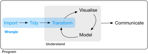
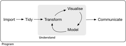
As the graphic implies, the data wrangling process includes data import, tidying, and transformation. The process directly feeds into, and is not mutually exclusive, with the understanding or modelling side of data exploration. More generally, I consider data wrangling as the manipulation or combination of datasets for the purpose of analysis.
Wrangling begins with import and ends with an output of some kind, such as a plot or a model. In a perfect world, the wrangling process is linear with no need for back-tracking. In reality, we often uncover more information about a dataset, either through wrangling or modeling, that warrants re-evaluation or even gathering more data. Data also come in many forms and the form you need for analysis is rarely the required form of the input data. For these reasons, data wrangling will consume most of your time in data exploration.
All wrangling is based on a purpose. No one wrangles for the sake of wrangling (usually), so the process always begins by answering the following two questions:
- What do my input data look like?
- What should my input data look like given what I want to do?
At the most basic level, going from what your data looks like to what it should look like will require a few key operations. Some common examples:
- Selecting specific variables
- Filtering observations by some criteria
- Adding or modifying existing variables
- Renaming variables
- Arranging rows by a variable
- Summarizing variable conditional on others
The dplyr package provides easy tools for these common data manipulation tasks. It is built to work directly with data frames and this is one of the foundational packages in what is now known as the tidyverse. The philosophy of dplyr is that one function does one thing and the name of the function says what it does. This is where the tidyverse generally departs from other packages and even base R. It is meant to be easy, logical, and intuitive. There is a lot of great info on dplyr. If you have an interest, I’d encourage you to look more. The vignettes are particularly good.
I’ll demonstrate the examples with the mpg dataset from last time. This dataset describes fuel economy of different vehicles and it comes with the tidyverse. Let’s get a feel for the data.
# convert to data frame, just cause
mpg <- as.data.frame(mpg)

# see first six rows
head(mpg)
## manufacturer model displ year cyl trans drv cty hwy fl class
## 1 audi a4 1.8 1999 4 auto(l5) f 18 29 p compact
## 2 audi a4 1.8 1999 4 manual(m5) f 21 29 p compact
## 3 audi a4 2.0 2008 4 manual(m6) f 20 31 p compact
## 4 audi a4 2.0 2008 4 auto(av) f 21 30 p compact
## 5 audi a4 2.8 1999 6 auto(l5) f 16 26 p compact
## 6 audi a4 2.8 1999 6 manual(m5) f 18 26 p compact# dimensions
dim(mpg)## [1] 234 11# column names
names(mpg)## [1] "manufacturer" "model" "displ" "year"
## [5] "cyl" "trans" "drv" "cty"
## [9] "hwy" "fl" "class"# structure
str(mpg)## 'data.frame': 234 obs. of 11 variables:
## $ manufacturer: chr "audi" "audi" "audi" "audi" ...
## $ model : chr "a4" "a4" "a4" "a4" ...
## $ displ : num 1.8 1.8 2 2 2.8 2.8 3.1 1.8 1.8 2 ...
## $ year : int 1999 1999 2008 2008 1999 1999 2008 1999 1999 2008 ...
## $ cyl : int 4 4 4 4 6 6 6 4 4 4 ...
## $ trans : chr "auto(l5)" "manual(m5)" "manual(m6)" "auto(av)" ...
## $ drv : chr "f" "f" "f" "f" ...
## $ cty : int 18 21 20 21 16 18 18 18 16 20 ...
## $ hwy : int 29 29 31 30 26 26 27 26 25 28 ...
## $ fl : chr "p" "p" "p" "p" ...
## $ class : chr "compact" "compact" "compact" "compact" ...Selecting
Let’s begin using dplyr. Don’t forget to load the tidyverse if you haven’t done so already.
# first, select some columns
dplyr_sel1 <- select(mpg, manufacturer, model, cty, hwy)
head(dplyr_sel1)
## manufacturer model cty hwy
## 1 audi a4 18 29
## 2 audi a4 21 29
## 3 audi a4 20 31
## 4 audi a4 21 30
## 5 audi a4 16 26
## 6 audi a4 18 26# select everything but class and drv
dplyr_sel2 <- select(mpg, -drv, -class)
head(dplyr_sel2)## manufacturer model displ year cyl trans cty hwy fl
## 1 audi a4 1.8 1999 4 auto(l5) 18 29 p
## 2 audi a4 1.8 1999 4 manual(m5) 21 29 p
## 3 audi a4 2.0 2008 4 manual(m6) 20 31 p
## 4 audi a4 2.0 2008 4 auto(av) 21 30 p
## 5 audi a4 2.8 1999 6 auto(l5) 16 26 p
## 6 audi a4 2.8 1999 6 manual(m5) 18 26 p# select columns that contain the letter c
dplyr_sel3 <- select(mpg, matches('c'))
head(dplyr_sel3)## manufacturer cyl cty class
## 1 audi 4 18 compact
## 2 audi 4 21 compact
## 3 audi 4 20 compact
## 4 audi 4 21 compact
## 5 audi 6 16 compact
## 6 audi 6 18 compactFiltering
After selecting columns, you’ll probably want to remove observations that don’t fit some criteria. For example, maybe you want to remove all cars from the dataset that have low mileage on the highway. Maybe you want to look at only six cylinder cars.
# now select (filter) some observations
dplyr_good_fuel <- filter(mpg, hwy > 25)
head(dplyr_good_fuel)
## manufacturer model displ year cyl trans drv cty hwy fl class
## 1 audi a4 1.8 1999 4 auto(l5) f 18 29 p compact
## 2 audi a4 1.8 1999 4 manual(m5) f 21 29 p compact
## 3 audi a4 2.0 2008 4 manual(m6) f 20 31 p compact
## 4 audi a4 2.0 2008 4 auto(av) f 21 30 p compact
## 5 audi a4 2.8 1999 6 auto(l5) f 16 26 p compact
## 6 audi a4 2.8 1999 6 manual(m5) f 18 26 p compact# now select observations for only six cylinder vehicles
dplyr_six_cyl <- filter(mpg, cyl == 6)
head(dplyr_six_cyl)## manufacturer model displ year cyl trans drv cty hwy fl class
## 1 audi a4 2.8 1999 6 auto(l5) f 16 26 p compact
## 2 audi a4 2.8 1999 6 manual(m5) f 18 26 p compact
## 3 audi a4 3.1 2008 6 auto(av) f 18 27 p compact
## 4 audi a4 quattro 2.8 1999 6 auto(l5) 4 15 25 p compact
## 5 audi a4 quattro 2.8 1999 6 manual(m5) 4 17 25 p compact
## 6 audi a4 quattro 3.1 2008 6 auto(s6) 4 17 25 p compactFiltering can take a bit of time to master because there are several ways to tell R what you want. Within the filter function, the working part is a logical selection of TRUE and FALSE values that are used to selected rows (TRUE means I want that row, FALSE means I don’t). Every selection within the filter function, no matter how complicated, will always be a T/F vector. This is similar to running queries on a database if you’re familiar with SQL.
To use filtering effectively, you have to know how to select the observations that you want using the comparison operators. R provides the standard suite: >, >=, <, <=, != (not equal), and == (equal). When you’re starting out with R, the easiest mistake to make is to use = instead of == when testing for equality.
Multiple arguments to filter() are combined with “and”: every expression must be true in order for a row to be included in the output. For other types of combinations, you’ll need to use Boolean operators yourself: & is “and”, | is “or”, and ! is “not”. This is the complete set of Boolean operations.
![]()
Let’s start combining filtering operations.
# get cars with city mileage betwen 18 and 22
filt1 <- filter(mpg, cty > 18 & cty < 22)
head(filt1)
## manufacturer model displ year cyl trans drv cty hwy fl class
## 1 audi a4 1.8 1999 4 manual(m5) f 21 29 p compact
## 2 audi a4 2.0 2008 4 manual(m6) f 20 31 p compact
## 3 audi a4 2.0 2008 4 auto(av) f 21 30 p compact
## 4 audi a4 quattro 2.0 2008 4 manual(m6) 4 20 28 p compact
## 5 audi a4 quattro 2.0 2008 4 auto(s6) 4 19 27 p compact
## 6 chevrolet malibu 2.4 1999 4 auto(l4) f 19 27 r midsize# get four cylinder or compact cars
filt2 <- filter(mpg, cyl == 4 | class == 'compact')
head(filt2)## manufacturer model displ year cyl trans drv cty hwy fl class
## 1 audi a4 1.8 1999 4 auto(l5) f 18 29 p compact
## 2 audi a4 1.8 1999 4 manual(m5) f 21 29 p compact
## 3 audi a4 2.0 2008 4 manual(m6) f 20 31 p compact
## 4 audi a4 2.0 2008 4 auto(av) f 21 30 p compact
## 5 audi a4 2.8 1999 6 auto(l5) f 16 26 p compact
## 6 audi a4 2.8 1999 6 manual(m5) f 18 26 p compact# get four cylinder and compact cars
filt3 <- filter(mpg, cyl == 4 & class == 'compact')
head(filt3)## manufacturer model displ year cyl trans drv cty hwy fl class
## 1 audi a4 1.8 1999 4 auto(l5) f 18 29 p compact
## 2 audi a4 1.8 1999 4 manual(m5) f 21 29 p compact
## 3 audi a4 2.0 2008 4 manual(m6) f 20 31 p compact
## 4 audi a4 2.0 2008 4 auto(av) f 21 30 p compact
## 5 audi a4 quattro 1.8 1999 4 manual(m5) 4 18 26 p compact
## 6 audi a4 quattro 1.8 1999 4 auto(l5) 4 16 25 p compact# get cars manufactured by ford or toyota
filt4 <- filter(mpg, manufacturer == 'ford' | manufacturer == 'toyota')
head(filt4)## manufacturer model displ year cyl trans drv cty hwy fl
## 1 ford expedition 2wd 4.6 1999 8 auto(l4) r 11 17 r
## 2 ford expedition 2wd 5.4 1999 8 auto(l4) r 11 17 r
## 3 ford expedition 2wd 5.4 2008 8 auto(l6) r 12 18 r
## 4 ford explorer 4wd 4.0 1999 6 auto(l5) 4 14 17 r
## 5 ford explorer 4wd 4.0 1999 6 manual(m5) 4 15 19 r
## 6 ford explorer 4wd 4.0 1999 6 auto(l5) 4 14 17 r
## class
## 1 suv
## 2 suv
## 3 suv
## 4 suv
## 5 suv
## 6 suv# an alternative way to get ford and toyota
filt5 <- filter(mpg, manufacturer %in% c('ford', 'toyota'))
head(filt5)## manufacturer model displ year cyl trans drv cty hwy fl
## 1 ford expedition 2wd 4.6 1999 8 auto(l4) r 11 17 r
## 2 ford expedition 2wd 5.4 1999 8 auto(l4) r 11 17 r
## 3 ford expedition 2wd 5.4 2008 8 auto(l6) r 12 18 r
## 4 ford explorer 4wd 4.0 1999 6 auto(l5) 4 14 17 r
## 5 ford explorer 4wd 4.0 1999 6 manual(m5) 4 15 19 r
## 6 ford explorer 4wd 4.0 1999 6 auto(l5) 4 14 17 r
## class
## 1 suv
## 2 suv
## 3 suv
## 4 suv
## 5 suv
## 6 suvMutating
Now that we’ve seen how to filter observations and select columns of a data frame, maybe we want to add a new column. In dplyr, mutate allows us to add new columns. These can be vectors you are adding or based on expressions applied to existing columns. For instance, we have a column of highway mileage and maybe we want to convert to km/l (Google says the conversion factor is 0.425).
# add a column for km/L
dplyr_mut <- mutate(mpg, hwy_kml = hwy * 0.425)
head(dplyr_mut)
## manufacturer model displ year cyl trans drv cty hwy fl class
## 1 audi a4 1.8 1999 4 auto(l5) f 18 29 p compact
## 2 audi a4 1.8 1999 4 manual(m5) f 21 29 p compact
## 3 audi a4 2.0 2008 4 manual(m6) f 20 31 p compact
## 4 audi a4 2.0 2008 4 auto(av) f 21 30 p compact
## 5 audi a4 2.8 1999 6 auto(l5) f 16 26 p compact
## 6 audi a4 2.8 1999 6 manual(m5) f 18 26 p compact
## hwy_kml
## 1 12.325
## 2 12.325
## 3 13.175
## 4 12.750
## 5 11.050
## 6 11.050# add a column for lo/hi fuel economy
dplyr_mut2 <- mutate(mpg, hwy_cat = ifelse(hwy < 25, 'hi', 'lo'))
head(dplyr_mut2)## manufacturer model displ year cyl trans drv cty hwy fl class
## 1 audi a4 1.8 1999 4 auto(l5) f 18 29 p compact
## 2 audi a4 1.8 1999 4 manual(m5) f 21 29 p compact
## 3 audi a4 2.0 2008 4 manual(m6) f 20 31 p compact
## 4 audi a4 2.0 2008 4 auto(av) f 21 30 p compact
## 5 audi a4 2.8 1999 6 auto(l5) f 16 26 p compact
## 6 audi a4 2.8 1999 6 manual(m5) f 18 26 p compact
## hwy_cat
## 1 lo
## 2 lo
## 3 lo
## 4 lo
## 5 lo
## 6 loSome other useful dplyr functions include arrange to sort the observations (rows) by a column and rename to (you guessed it) rename a column.
# arrange by highway economy
dplyr_arr <- arrange(mpg, hwy)
head(dplyr_arr)
## manufacturer model displ year cyl trans drv cty hwy
## 1 dodge dakota pickup 4wd 4.7 2008 8 auto(l5) 4 9 12
## 2 dodge durango 4wd 4.7 2008 8 auto(l5) 4 9 12
## 3 dodge ram 1500 pickup 4wd 4.7 2008 8 auto(l5) 4 9 12
## 4 dodge ram 1500 pickup 4wd 4.7 2008 8 manual(m6) 4 9 12
## 5 jeep grand cherokee 4wd 4.7 2008 8 auto(l5) 4 9 12
## 6 chevrolet k1500 tahoe 4wd 5.3 2008 8 auto(l4) 4 11 14
## fl class
## 1 e pickup
## 2 e suv
## 3 e pickup
## 4 e pickup
## 5 e suv
## 6 e suv# rename some columns
dplyr_rnm <- rename(mpg, make = manufacturer)
head(dplyr_rnm)## make model displ year cyl trans drv cty hwy fl class
## 1 audi a4 1.8 1999 4 auto(l5) f 18 29 p compact
## 2 audi a4 1.8 1999 4 manual(m5) f 21 29 p compact
## 3 audi a4 2.0 2008 4 manual(m6) f 20 31 p compact
## 4 audi a4 2.0 2008 4 auto(av) f 21 30 p compact
## 5 audi a4 2.8 1999 6 auto(l5) f 16 26 p compact
## 6 audi a4 2.8 1999 6 manual(m5) f 18 26 p compactThere are many more functions in dplyr but the one’s above are by far the most used. As you can imagine, they are most effective when used to together because there is never only one step in the data wrangling process. After the exercise, we’ll talk about how we can efficiently pipe the functions in dplyr to create a new data object.
Exercise 2
Now that you know the basic functions in dplyr and how to use them, let’s apply them to a more relevant dataset. We’re going to import the sediment chemistry dataset from Bight13 and grab some specific data that we want. We’ll be getting all of the observations for chlorophyll (Total_CHL) and organic carbon (Total Organic Carbon). We’ll remove everything else in the data that we don’t need.
Import the Bight chemistry data using the
read_excelfunction from the readxl package. The data should be in yourdatafolder. Make sure to store it as an object in your workspace (use<-).Now we need to think about what variables we need to get the chlorophyll data. Select the
StationID,Parameter, andResultcolumns and assign it as a new object in your environment.Using the new object, let’s filter the observations (i.e., the
Parametercolumn) to get only chlorophyll (Total_CHL) and organic carbon (Total Organic Carbon). Again, assign the new object to your environment.When you’re happy with the result, have a look at the data. Did you get what you wanted? How many observations do you have compared to the original data file? Did you succesfully filter the right parameters (hint:
table(dat$Parameter)?Save the new file to your data folder using
write_csvand call itBight_wrangle.csv. Don’t forget to include the full path within your project when saving the file.
Piping
A complete data wrangling exercise will always include multiple steps to go from the raw data to the output you need. Here’s a terrible wrangling example using functions from base R:
cropdat <- rawdat[1:28]
savecols <- data.frame(cropdat$Party, cropdat$`Last Inventory Year (2015)`)
names(savecols) <- c('Party','2015')
savecols$rank2015 <- rank(-savecols$`2015`)
top10df <- savecols[savecols$rank2015 <= 10,]
basedat <- cropdat[cropdat$Party %in% top10df$Party,]
Technically, if this works it’s not “wrong”, but there are a couple issues that can lead to problems down the line. First, the flow of functions to manipulate the data is not obvious and this makes your code very hard to read. Second, lots of unecessary intermediates have been created in your workspace. Anything that adds to clutter should be avoided because R is fundamentally based on object assignments. The less you assign as a variable in your environment the easier it will be to navigate complex scripts.
The good news is that you now know how to use the dplyr functions to wrangle data. The function names in dplyr were chosen specifically to be descriptive. This will make your code much more readable than if you were using base R counterparts. The bad news is that I haven’t told you how to easily link the functions. Fortunately, there’s an easy fix to this problem.
The magrittr package (comes with tidyverse) provides a very useful method called piping that will make wrangling a whole lot easier. The idea is simple: a pipe (%>%) is used to chain functions together. The output from one function becomes the input to the next function in the pipe. This avoids the need to create intermediate objects and creates a logical progression of steps that demystify the wrangling process.
Consider the simple example:
# not using pipes, select a column, filter rows
bad_ex <- select(mpg, manufacturer, hwy)
bad_ex2 <- filter(bad_ex, hwy > 25)
With pipes, it looks like this:
# with pipes, select a column, filter rows
good_ex <- select(mpg, manufacturer, hwy) %>%
  filter(hwy > 25)
Now we’ve created only one new object in our environment and we can clearly see that we select, then filter. The only real coding difference is now the filter function only includes the part about which rows to keep. You do not need to specify a data object as input to a function if you’re using piping. The pipe will always use the input that comes from above.
Using pipes, you can link together as many functions as you like.
# a complete piping example
all_pipes <- mpg %>%
  select(manufacturer, year, hwy, cty) %>%
  filter(year == 2008 & hwy <= 25) %>%
  rename(
    make = manufacturer,
    hmpg = hwy,
    cmpg = cty
    ) %>%
  arrange(-hmpg)
head(all_pipes)
## make year hmpg cmpg
## 1 audi 2008 25 17
## 2 audi 2008 25 15
## 3 audi 2008 25 17
## 4 chevrolet 2008 25 15
## 5 nissan 2008 25 19
## 6 pontiac 2008 25 16A couple comments about piping:
- I find it very annoying to type the pipe operator (six key strokes!). RStudio has a nice keyboard shortcut:
Crtl + Shift + Mfor Windows (useCmd + Shift + Mon a mac). - It’s convention to start a new function on the next line after a pipe operator. This makes the code easier to read and you can also comment out a single step in a long pipe.
- Don’t make your pipes too long, limit them to a particular data object or task.
Exercise 3
Now that we know how to pipe functions, let’s repeat exercise 2 with the Bight data. You should already have code to import, select, and filter the data. In theory, you could create all of exercise 2 with a single continuous pipe. That’s a bit excessive so try to do this by creating only two objects in your workspace. Make one object the raw data and the second object the wrangled data.
- Using your code from exercise two, try to replicate the steps using pipes. The steps we used in exercise two were:
- Import the raw data with
read_excel - Select the columns
StationID,Parameter, andResult - Filter parameter to get only
Total_CHLandTotal Organic Carbon(hint: use%in%)
- Import the raw data with
- When you’re done, you should have a data object that’s exactly the same as the one you created in exercise two. Try to verify this with the
identicalfunction from base R (check the help file with?identicalif you don’t know how to use this function).
Next time
Now you should be able to answer (or be able to find answers to) the following:
- Why do we need to manipulate data?
- What is the tidyverse?
- What can you do with dplyr?
- What is piping?
Next time we’ll continue with data wrangling.
Attribution
Content in this lesson was pillaged extensively from the USGS-R training curriculum here and R for data Science.