README

Install the package as follows:

install.packages('devtools')
library(devtools)
install_github('SCCWRP/SQObioaccumulation')
library(SQObioaccumulation)

Run the bioaccumulation model with defaults:

# data inputs
data(biota)
data(constants)
data(contam)
data(mcsparms)

# calculated contaminant inputs
contamcalc <- cntcalc(contam, constants)

# run model
res <- bioaccum_batch(biota, contamcalc, constants)

# assign output to separate objects
cbiota <- res$cbiota
bsaf <- res$bsaf

Creat a summary table:

# summary table
indic_sum <- indic_sum_fun(cbiota, contamcalc)
indic_sum

## # A tibble: 9 x 9
##   Guild `Chlordanes BSA~ `Dieldrin BSAF ~ `DDTs BSAF (cal~ `PCBs BSAF (cal~
##   <chr>            <dbl>            <dbl>            <dbl>            <dbl>
## 1 indi~             5.30            2.10             11.2              9.13
## 2 indi~             5.45            1.99             12.4             10.0 
## 3 indi~             5.26            2.25              9.55             7.93
## 4 indi~             6.33            3.22             13.0             11.1 
## 5 indi~             2.28            1.21              4.43             3.84
## 6 indi~             5.42            3.89              7.30             6.64
## 7 indi~             1.40            0.924             2.05             1.84
## 8 indi~             4.15            3.71              3.98             4.03
## 9 indi~             4.75            1.70             11.6              9.32
## # ... with 4 more variables: `Chlordanes Conc (ng/g)` <dbl>, `Dieldrin
## #   Conc (ng/g)` <dbl>, `DDTs Conc (ng/g)` <dbl>, `PCBs Conc (ng/g)` <dbl>

Plot BSAF and tissue concentration estimates for a selected contaminant:

# plot of bsaf, cbiota by specific contaminant
plo_bsaf(bsaf, cbiota, 'alphaChlordane')

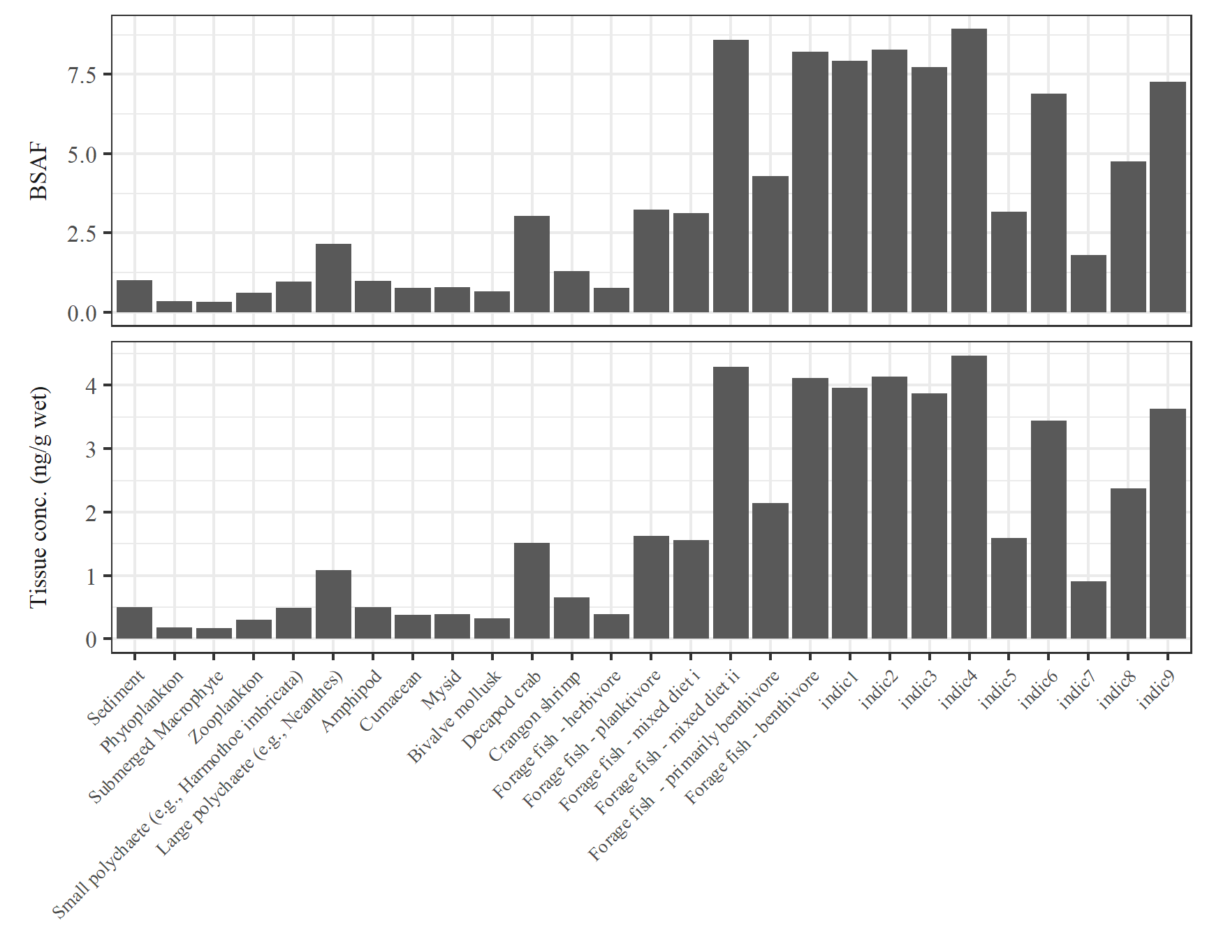
Make a table of BSAF and tissue concentration estimates for a selected contaminant:

# tabular summary of bsaf, cbiota by specific contaminant
tab_bsaf(bsaf, cbiota, 'alphaChlordane')

## # A tibble: 2 x 28
##   Output Sediment Phytoplankton `Submerged Macr~ Zooplankton
##   <fct>     <dbl>         <dbl>            <dbl>       <dbl>
## 1 Tissu~      0.5         0.177            0.166       0.302
## 2 BSAF        1           0.355            0.331       0.605
## # ... with 23 more variables: `Small polychaete (e.g., Harmothoe
## #   imbricata)` <dbl>, `Large polychaete (e.g., Neanthes)` <dbl>,
## #   Amphipod <dbl>, Cumacean <dbl>, Mysid <dbl>, `Bivalve mollusk` <dbl>,
## #   `Decapod crab` <dbl>, `Crangon shrimp` <dbl>, `Forage fish -
## #   herbivore` <dbl>, `Forage fish - planktivore` <dbl>, `Forage fish -
## #   mixed diet i` <dbl>, `Forage fish - mixed diet ii` <dbl>, `Forage fish
## #   - primarily benthivore` <dbl>, `Forage fish - benthivore` <dbl>,
## #   indic1 <dbl>, indic2 <dbl>, indic3 <dbl>, indic4 <dbl>, indic5 <dbl>,
## #   indic6 <dbl>, indic7 <dbl>, indic8 <dbl>, indic9 <dbl>

Run Monte Carlo simulations (MCS) with results from bioaccumulation model and additional inputs:

mcsres <- mcs_fun(1000, indic_sum, mcsparms, constants)

Summarize MCS results:

mcs_sum_fun(mcsres)

## # A tibble: 4 x 12
## # Groups:   Compound [4]
##   Compound    `0%`    `1%`   `5%`  `10%`  `25%` `50%` `75%` `90%` `95%`
##   <chr>      <dbl>   <dbl>  <dbl>  <dbl>  <dbl> <dbl> <dbl> <dbl> <dbl>
## 1 Chlorda~ 0.158   0.219   0.292  0.358  0.523  0.761 1.07  1.52   1.91
## 2 DDT      0.121   0.209   0.389  0.503  0.869  1.55  2.80  4.72   6.55
## 3 Dieldrin 0.554   0.841   1.18   1.42   1.97   2.77  3.94  5.41   6.45
## 4 PCB      0.00525 0.00859 0.0208 0.0333 0.0732 0.158 0.368 0.718  1.09
## # ... with 2 more variables: `99%` <dbl>, `100%` <dbl>

Plot cumulative distribution curves for MCS:

mcs_plo(mcsres, xmax = 3)

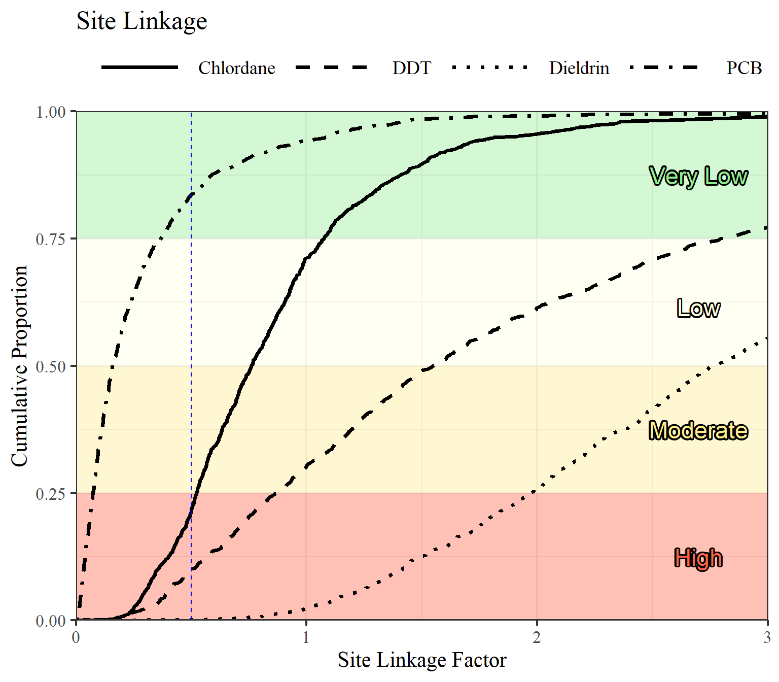
Get overall SQO assessment:

wgtavg <- wgt_avg_fun(mcsparms)
sqo_sum_fun(wgtavg, mcsres, constants)

## # A tibble: 4 x 9
##   Compound `Observed tissu~ `Chemical expos~ `Estimated tiss~
##   <chr>               <dbl> <chr>                       <dbl>
## 1 Chlorda~             2.28 Very Low                    1.74 
## 2 DDT                  4.85 Very Low                    7.52 
## 3 Dieldrin             0.25 Very Low                    0.693
## 4 PCB                 36.5  Moderate                    5.77 
## # ... with 5 more variables: `Site linkage 25%` <dbl>, `Site linkage
## #   50%` <dbl>, `Site linkage 75%` <dbl>, `Site linkage category` <chr>,
## #   `Site assessment category` <chr>