Wrangling and plotting data in R
Lesson Outline
Lesson Exercises
Goals and Motivation
Data wrangling (manipulation, cleaning, ninjery, etc.) is the part of any data analysis that will take the most time. While it may not necessarily be fun, it is foundational to all the work that follows. I strongly believe that mastering these skills has more value than mastering a particular analysis. Check out this article if you don’t believe me. Creating a data visualization will always begin with wrangling, so we’ll cover some core wrangling concepts first before we start plotting.
After this session you should be able answer the following:
- What are some basic wrangling functions from dplyr?
- How do I join different datasets?
- How do I make some basic plots with ggplot?
Data wrangling with dplyr

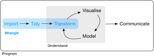
The data wrangling process includes data import, tidying, and transformation. The process directly feeds into, and is not mutually exclusive with, the understanding or modelling side of data exploration. More generally, I consider data wrangling as the manipulation or combination of datasets for the purpose of analysis.
All wrangling is based on a purpose. No one wrangles for the sake of wrangling (usually), so the process always begins by answering the following two questions:
- What do my input data look like?
- What should my input data look like given what I want to do?
At the most basic level, going from what your data looks like to what it should look like will require a few key operations. Some common examples:
- Selecting specific variables
- Filtering observations by some criteria
- Adding or modifying existing variables
- Renaming variables
- Arranging rows by a variable
- Summarizing a variable conditional on others
The dplyr package provides easy tools for these common data manipulation tasks and is a core package from the tidyverse suite of packages. The philosophy of dplyr is that one function does one thing and the name of the function says what it does. Some additional dplyr resources:
Exercise 1
We’ll start this lesson by opening a clean script, loading the packages we need, and importing our data.
Open a new script from the file menu on the top left and save the script with an informative name, e.g., “wrangling_and_plotting.R”.
Add in a comment line on the top and write some text about the script. It should look something like:
# Exercise 2: Wrangling and plotting bioassessment data.Below the comment line, add the code to import the tidyverse, i.e.,
library(tidyverse).In the next line, add the following to import our two datasets.
cscidat <- read.csv('data/cscidat.csv', stringsAsFactors = F)
ascidat <- read.csv('data/ascidat.csv', stringsAsFactors = F)
When you’re done, run all of the code in the console (highlight all then
ctrl+enter)
Our goal with these data is to combine the bioassessment scores by each unique location, date, and replicate, while keeping only the data we need for our plots.
Selecting
Let’s begin using dplyr. The select function lets you retain or exclude columns.
# first, select some columns
dplyr_sel1 <- select(cscidat, SampleID_old, New_Lat, New_Long, CSCI)
head(dplyr_sel1)
## SampleID_old New_Lat New_Long CSCI
## 1 000CAT148_8.10.10_1 39.07523 -119.8994 0.9879779
## 2 000CAT228_8.10.10_1 39.07307 -119.9201 0.9811505
## 3 102PS0139_8.9.10_1 41.99595 -122.9597 1.0715694
## 4 103CDCHHR_9.14.10_1 41.78890 -124.0778 1.0866419
## 5 103FC1106_7.15.14_1 41.93407 -124.1081 0.9971599
## 6 103FCA168_7.24.13_1 41.64962 -124.0912 1.0633122# select everything but CSCI and COMID
dplyr_sel2 <- select(cscidat, -CSCI, -COMID)
head(dplyr_sel2)## SampleID_old StationCode New_Lat New_Long E OE
## 1 000CAT148_8.10.10_1 000CAT148 39.07523 -119.8994 16.05804 0.9309977
## 2 000CAT228_8.10.10_1 000CAT228 39.07307 -119.9201 16.08960 0.9726777
## 3 102PS0139_8.9.10_1 102PS0139 41.99595 -122.9597 15.46439 1.0896002
## 4 103CDCHHR_9.14.10_1 103CDCHHR 41.78890 -124.0778 21.10443 1.0898184
## 5 103FC1106_7.15.14_1 103FC1106 41.93407 -124.1081 16.83757 1.0779468
## 6 103FCA168_7.24.13_1 103FCA168 41.64962 -124.0912 19.07408 1.0931064
## pMMI SampleID_old.1
## 1 1.0449580 000CAT148_8.10.10_1
## 2 0.9896232 000CAT228_8.10.10_1
## 3 1.0535386 102PS0139_8.9.10_1
## 4 1.0834653 103CDCHHR_9.14.10_1
## 5 0.9163731 103FC1106_7.15.14_1
## 6 1.0335179 103FCA168_7.24.13_1# select columns that contain the letter c
dplyr_sel3 <- select(cscidat, matches('c'))
head(dplyr_sel3)## StationCode COMID CSCI
## 1 000CAT148 8942501 0.9879779
## 2 000CAT228 8942503 0.9811505
## 3 102PS0139 23936337 1.0715694
## 4 103CDCHHR 22226836 1.0866419
## 5 103FC1106 22226634 0.9971599
## 6 103FCA168 22226990 1.0633122Filtering
After selecting columns, you’ll probably want to remove observations that don’t fit some criteria. For example, maybe you want to remove CSCI scores less than some threshold, find stations above a certain latitude, or both.
# get CSCI scores greater than 0.79
dplyr_filt1 <- filter(cscidat, CSCI > 0.79)
head(dplyr_filt1)
## SampleID_old StationCode New_Lat New_Long COMID E
## 1 000CAT148_8.10.10_1 000CAT148 39.07523 -119.8994 8942501 16.05804
## 2 000CAT228_8.10.10_1 000CAT228 39.07307 -119.9201 8942503 16.08960
## 3 102PS0139_8.9.10_1 102PS0139 41.99595 -122.9597 23936337 15.46439
## 4 103CDCHHR_9.14.10_1 103CDCHHR 41.78890 -124.0778 22226836 21.10443
## 5 103FC1106_7.15.14_1 103FC1106 41.93407 -124.1081 22226634 16.83757
## 6 103FCA168_7.24.13_1 103FCA168 41.64962 -124.0912 22226990 19.07408
## OE pMMI CSCI SampleID_old.1
## 1 0.9309977 1.0449580 0.9879779 000CAT148_8.10.10_1
## 2 0.9726777 0.9896232 0.9811505 000CAT228_8.10.10_1
## 3 1.0896002 1.0535386 1.0715694 102PS0139_8.9.10_1
## 4 1.0898184 1.0834653 1.0866419 103CDCHHR_9.14.10_1
## 5 1.0779468 0.9163731 0.9971599 103FC1106_7.15.14_1
## 6 1.0931064 1.0335179 1.0633122 103FCA168_7.24.13_1# get CSCI scores above latitude 37N
dplyr_filt2 <- filter(cscidat, New_Lat > 37)
head(dplyr_filt2)## SampleID_old StationCode New_Lat New_Long COMID E
## 1 000CAT148_8.10.10_1 000CAT148 39.07523 -119.8994 8942501 16.05804
## 2 000CAT228_8.10.10_1 000CAT228 39.07307 -119.9201 8942503 16.08960
## 3 102PS0139_8.9.10_1 102PS0139 41.99595 -122.9597 23936337 15.46439
## 4 103CDCHHR_9.14.10_1 103CDCHHR 41.78890 -124.0778 22226836 21.10443
## 5 103FC1106_7.15.14_1 103FC1106 41.93407 -124.1081 22226634 16.83757
## 6 103FCA168_7.24.13_1 103FCA168 41.64962 -124.0912 22226990 19.07408
## OE pMMI CSCI SampleID_old.1
## 1 0.9309977 1.0449580 0.9879779 000CAT148_8.10.10_1
## 2 0.9726777 0.9896232 0.9811505 000CAT228_8.10.10_1
## 3 1.0896002 1.0535386 1.0715694 102PS0139_8.9.10_1
## 4 1.0898184 1.0834653 1.0866419 103CDCHHR_9.14.10_1
## 5 1.0779468 0.9163731 0.9971599 103FC1106_7.15.14_1
## 6 1.0931064 1.0335179 1.0633122 103FCA168_7.24.13_1# use both filters
dplyr_filt3 <- filter(cscidat, CSCI > 0.79 & New_Lat > 37)
head(dplyr_filt3)## SampleID_old StationCode New_Lat New_Long COMID E
## 1 000CAT148_8.10.10_1 000CAT148 39.07523 -119.8994 8942501 16.05804
## 2 000CAT228_8.10.10_1 000CAT228 39.07307 -119.9201 8942503 16.08960
## 3 102PS0139_8.9.10_1 102PS0139 41.99595 -122.9597 23936337 15.46439
## 4 103CDCHHR_9.14.10_1 103CDCHHR 41.78890 -124.0778 22226836 21.10443
## 5 103FC1106_7.15.14_1 103FC1106 41.93407 -124.1081 22226634 16.83757
## 6 103FCA168_7.24.13_1 103FCA168 41.64962 -124.0912 22226990 19.07408
## OE pMMI CSCI SampleID_old.1
## 1 0.9309977 1.0449580 0.9879779 000CAT148_8.10.10_1
## 2 0.9726777 0.9896232 0.9811505 000CAT228_8.10.10_1
## 3 1.0896002 1.0535386 1.0715694 102PS0139_8.9.10_1
## 4 1.0898184 1.0834653 1.0866419 103CDCHHR_9.14.10_1
## 5 1.0779468 0.9163731 0.9971599 103FC1106_7.15.14_1
## 6 1.0931064 1.0335179 1.0633122 103FCA168_7.24.13_1Filtering can take a bit of time to master because there are several ways to tell R what you want. To use filtering effectively, you have to know how to select the observations that you want using the comparison operators. R provides the standard suite: >, >=, <, <=, != (not equal), and == (equal). When you’re starting out with R, the easiest mistake to make is to use = instead of == when testing for equality.
Mutating
Now that we’ve seen how to filter observations and select columns of a data frame, maybe we want to add a new column. In dplyr, mutate allows us to add new columns. These can be vectors you are adding or based on expressions applied to existing columns. For instance, maybe we want to convert a numeric column into a categorical using some criteria or maybe we want to make a new column based on some arithmetic on some other columns.
# get observed taxa
dplyr_mut1 <- mutate(cscidat, observed = OE * E)
head(dplyr_mut1)
## SampleID_old StationCode New_Lat New_Long COMID E
## 1 000CAT148_8.10.10_1 000CAT148 39.07523 -119.8994 8942501 16.05804
## 2 000CAT228_8.10.10_1 000CAT228 39.07307 -119.9201 8942503 16.08960
## 3 102PS0139_8.9.10_1 102PS0139 41.99595 -122.9597 23936337 15.46439
## 4 103CDCHHR_9.14.10_1 103CDCHHR 41.78890 -124.0778 22226836 21.10443
## 5 103FC1106_7.15.14_1 103FC1106 41.93407 -124.1081 22226634 16.83757
## 6 103FCA168_7.24.13_1 103FCA168 41.64962 -124.0912 22226990 19.07408
## OE pMMI CSCI SampleID_old.1 observed
## 1 0.9309977 1.0449580 0.9879779 000CAT148_8.10.10_1 14.95
## 2 0.9726777 0.9896232 0.9811505 000CAT228_8.10.10_1 15.65
## 3 1.0896002 1.0535386 1.0715694 102PS0139_8.9.10_1 16.85
## 4 1.0898184 1.0834653 1.0866419 103CDCHHR_9.14.10_1 23.00
## 5 1.0779468 0.9163731 0.9971599 103FC1106_7.15.14_1 18.15
## 6 1.0931064 1.0335179 1.0633122 103FCA168_7.24.13_1 20.85# add a column for lo/hi csci scores
dplyr_mut2 <- mutate(cscidat, CSCIcat = ifelse(CSCI <= 0.79, 'lo', 'hi'))
head(dplyr_mut2)## SampleID_old StationCode New_Lat New_Long COMID E
## 1 000CAT148_8.10.10_1 000CAT148 39.07523 -119.8994 8942501 16.05804
## 2 000CAT228_8.10.10_1 000CAT228 39.07307 -119.9201 8942503 16.08960
## 3 102PS0139_8.9.10_1 102PS0139 41.99595 -122.9597 23936337 15.46439
## 4 103CDCHHR_9.14.10_1 103CDCHHR 41.78890 -124.0778 22226836 21.10443
## 5 103FC1106_7.15.14_1 103FC1106 41.93407 -124.1081 22226634 16.83757
## 6 103FCA168_7.24.13_1 103FCA168 41.64962 -124.0912 22226990 19.07408
## OE pMMI CSCI SampleID_old.1 CSCIcat
## 1 0.9309977 1.0449580 0.9879779 000CAT148_8.10.10_1 hi
## 2 0.9726777 0.9896232 0.9811505 000CAT228_8.10.10_1 hi
## 3 1.0896002 1.0535386 1.0715694 102PS0139_8.9.10_1 hi
## 4 1.0898184 1.0834653 1.0866419 103CDCHHR_9.14.10_1 hi
## 5 1.0779468 0.9163731 0.9971599 103FC1106_7.15.14_1 hi
## 6 1.0931064 1.0335179 1.0633122 103FCA168_7.24.13_1 hiSome other useful dplyr functions include arrange to sort the observations (rows) by a column and rename to (you guessed it) rename a column.
# arrange by CSCI scores
dplyr_arr <- arrange(cscidat, CSCI)
head(dplyr_arr)
## SampleID_old StationCode New_Lat New_Long COMID E
## 1 206PS0073_7.20.10_1 206PS0073 38.09831 -122.5670 1669863 13.344409
## 2 205R01390_5.23.13_1 205R01390 37.53080 -121.9702 17692585 13.117454
## 3 205R00878_4.24.13_1 205R00878 37.55460 -121.9870 17691075 14.005475
## 4 801S03971_6.16.14_1 801S03971 33.67551 -117.8277 20355412 8.229786
## 5 204R00383_6.11.12_1 204R00383 37.65910 -122.1368 2804015 10.678176
## 6 204R00583_6.13.12_1 204R00583 37.61910 -122.0593 2804187 13.292084
## OE pMMI CSCI SampleID_old.1
## 1 0.1498755 0.0663000 0.1080869 206PS0073_7.20.10_1
## 2 0.1524686 0.0852000 0.1188203 205R01390_5.23.13_1
## 3 0.2142019 0.0336000 0.1239177 205R00878_4.24.13_1
## 4 0.0729000 0.2306298 0.1517679 801S03971_6.16.14_1
## 5 0.2809468 0.0325000 0.1567290 204R00383_6.11.12_1
## 6 0.2783612 0.0448000 0.1616011 204R00583_6.13.12_1# rename lat/lon (note the multiple arguments)
dplyr_rnm <- rename(cscidat,
lat = New_Lat,
lon = New_Long
)
head(dplyr_rnm)## SampleID_old StationCode lat lon COMID E
## 1 000CAT148_8.10.10_1 000CAT148 39.07523 -119.8994 8942501 16.05804
## 2 000CAT228_8.10.10_1 000CAT228 39.07307 -119.9201 8942503 16.08960
## 3 102PS0139_8.9.10_1 102PS0139 41.99595 -122.9597 23936337 15.46439
## 4 103CDCHHR_9.14.10_1 103CDCHHR 41.78890 -124.0778 22226836 21.10443
## 5 103FC1106_7.15.14_1 103FC1106 41.93407 -124.1081 22226634 16.83757
## 6 103FCA168_7.24.13_1 103FCA168 41.64962 -124.0912 22226990 19.07408
## OE pMMI CSCI SampleID_old.1
## 1 0.9309977 1.0449580 0.9879779 000CAT148_8.10.10_1
## 2 0.9726777 0.9896232 0.9811505 000CAT228_8.10.10_1
## 3 1.0896002 1.0535386 1.0715694 102PS0139_8.9.10_1
## 4 1.0898184 1.0834653 1.0866419 103CDCHHR_9.14.10_1
## 5 1.0779468 0.9163731 0.9971599 103FC1106_7.15.14_1
## 6 1.0931064 1.0335179 1.0633122 103FCA168_7.24.13_1Exercise 2
Let’s clean up our CSCI dataset in preparation to join with our ASCI dataset. We’ll select columns we want and rename those with odd names.
Select the unique sample ID column (
SampleID_old), latitude (New_Lat), longitude (New_Long), andCSCIcolumns. Reassign thecscidatdata object at the same time.cscidat <- select(cscidat, SampleID_old, New_Lat, New_Long, CSCI)Rename the
SampleID_oldcolumn toid,New_Lattolat, andNew_Longtolon.cscidat <- rename(cscidat, id = SampleID_old, lat = New_Lat, lon = New_Long )
Joining datasets
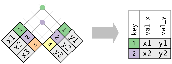
Combining data is a common task of data wrangling. All joins require that each of the tables can be linked by shared identifiers. These are called ‘keys’ and are usually represented as a separate column that acts as a unique variable for the observations. Our example datasets include the id column that represents a unique identifier as a combination of station, sample date, and replicate.
The challenge with joins is that the two datasets may not represent the same observations for a given key. For example, you might have one table with all observations for every key, another with only some observations, or two tables with only a few shared keys. What you get back from a join will depend on what’s shared between tables, in addition to the type of join you use.
For our data, we’ll be using an inner-join that combines datasets by shared keys (for an overview of the other types of joins, see here).

Exercise 3
We’ll join our ASCI data to our CSCI data in this exercise to make a single dataset that has scores for both bioassessment indices taken at the same place and time. This will help us plot and map the data later.
Before you start, check the dimensions of both datasets (e.g.,
dimornrow). How many rows in each?dim(cscidat) dim(ascidat)Using the
inner_joinfunction from dplyr, joincscidatwithascidatusing theidcolumn as the key.alldat <- inner_join(cscidat, ascidat, by = 'id')What are the dimensions of the new dataset (i.e., how many unique bioassessment scores were collected at the same time and place)?
Plotting with ggplot2
The entire workflow of data exploration is enhanced through looking at your data, whether you’re exploring a dataset for the first time or creating publication-ready figures. Viewing your data provides insight into patterns that can help you explore different hypotheses. No analysis is complete without a solid graphic.
We’ll only introduce some of the core concepts behind the popular ggplot2 package. This package follows a strict philosophy known as the grammar of graphics that was designed to make thinking, reasoning, and communicating about graphs easier by following a few simple rules. Like building a sentence in speech (aka grammar), all graphs start with a foundational component that is used for building other graph pieces.
With ggplot2, you begin a plot with the function ggplot(). ggplot() creates a coordinate system that you can add layers to. The first argument of ggplot() is the dataset to use in the graph. So ggplot(data = alldat) creates an empty base graph.
ggplot(data = alldat)You complete your graph by adding one or more layers (aka geoms) to ggplot(). The function geom_point() adds a layer of points to your plot, which creates a scatterplot. Ggplot2 comes with many geom functions that each add a different type of layer to a plot.
ggplot(data = alldat) +
  geom_point()
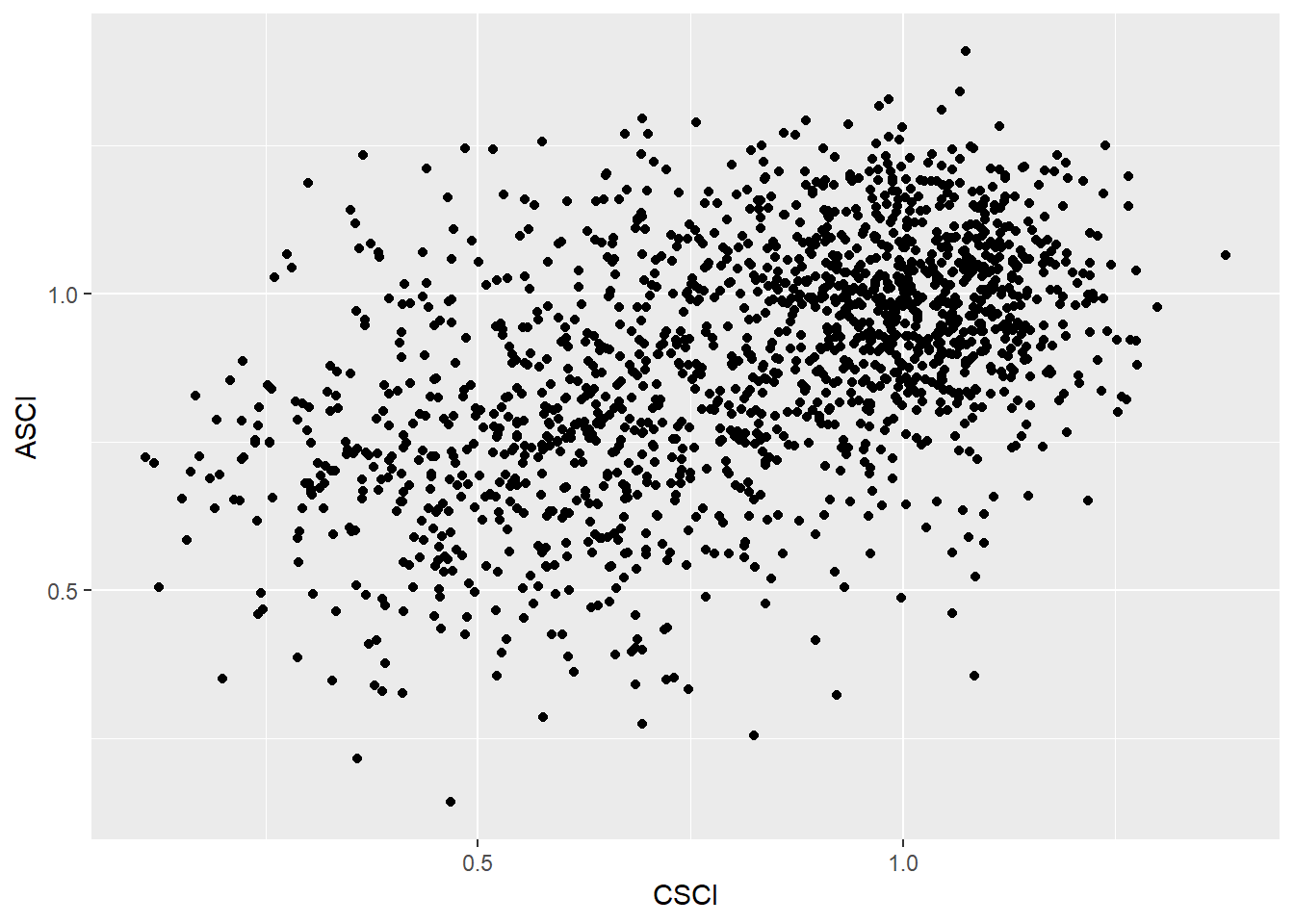
Each geom function in ggplot2 takes a mapping argument. This defines how variables in your dataset are mapped to visual properties. The mapping argument is defined with aes(), and the x and y arguments of aes() specify which variables to map to the x and y axes. ggplot2 looks for the mapped variable in the data argument, in this case, alldat.
ggplot(data = alldat) +
  geom_point(mapping = aes(x = CSCI, y = ASCI))
Just remember these requirements:
- All ggplot plots start with the
ggplotfunction - It will need three pieces of information: the data, how the data are mapped to the plot aesthetics, and a geom layer
The core unit of every ggplot looks like this:
ggplot(data = <DATA>) +
  <GEOM_FUNCTION>(mapping = aes(<MAPPINGS>))
Applied to the data:
ggplot(data = alldat) +
  geom_point(mapping = aes(x = CSCI, y = ASCI))
Exercise 4
Let’s make a quick ggplot using some of the guidance from above. In this example, we’ll create some boxplots to show the distribution of CSCI scores at different site types (i.e., reference, intermediate, and stressed). This follows the same syntax as above but we’ll use a categorical variable for the x aesthetic and use the geom_boxplot geometry.
Copy the code from the last example plot to your script.
Replace the
geom_pointfunction withgeom_boxplotMap the
site_typecolumn to the x aesthetic and theCSCIscores to the y aesthetic. The final code should look like this:ggplot(data = alldat) + geom_boxplot(mapping = aes(x = site_type, y = CSCI))When you’re done, run the code in the console and view the plot. What does it tell you about the distribution of CSCI scores?
There’s certainly much, much more we can do with ggplot2. Feel free to checkout the official ggplot2 website for more information. The RStudio cheatsheet is also very helpful.