Landsat Kelp Area Time Series • KelpAreaIndicator

Data setup and prerequisites

Install the KelpAreaIndicator package from the SCCWRP github repository and load it.

# devtools::install_github(
#   "SCCWRP/KelpAreaIndicator",
#   build_vignettes = TRUE,
#   build_manual = TRUE
# )
library(KelpAreaIndicator)

Provide the file paths to the Landsat kelp area data, downloaded from the EDI Data Portal, and the shapefile that defines the kelp segment polygons of interest. The kelp segments shapefile is a polygon shapefile with at least one attribute, Segment_ID, that defines the kelp area segments of interest with the WGS 84 CRS (EPSG:4326).

lter_file_path <- "../data/LandsatKelpBiomass_2024_Q2_withmetadata.nc"
kelp_segments_file_path <- "../data/uswc_2024_v2"

Assigning segments to Landsat pixels

The segment_landsat_data() function will load the Landsat netCDF file and assign each pixel to its respective segment, defined in the kelp segments shapefile. Each pixel in the Landsat data represents a 900 m $^2$ area, so the segment_landsat_data() function provides an option to treat the area values as either 0 or 900 m $^2$ , rather than the fractional value between 0 and 900, with the fractional_pixels parameter. Setting fractional_pixels = FALSE will enable this binary treatment of the pixel data.

The resulting data frame consists of rows of pixels from the Landsat data, and columns of quarters for each year of the time series. The Segment_ID column indicates which segment that the pixel belongs to. The lon and lat columns are the longitude and latitude of the pixel, respectively. The remaining columns represent the quarterly kelp area time series of that pixel, in m $^2$ .

segmented_landsat_data <- segment_landsat_data(
  lter_file_path = lter_file_path,
  kelp_segments_file_path = kelp_segments_file_path
)
#> Reading layer `uswc_2024_v2' from data source 
#>   `/Users/nicholasl/Documents/Projects/kelp/KelpAreaIndicator/data/uswc_2024_v2' 
#>   using driver `ESRI Shapefile'
#> Simple feature collection with 311 features and 1 field
#> Geometry type: POLYGON
#> Dimension:     XY
#> Bounding box:  xmin: -124.844 ymin: 32.52884 xmax: -117.1165 ymax: 48.42642
#> Geodetic CRS:  WGS 84

segmented_landsat_data
#> # A tibble: 382,462 × 165
#>    Segment_ID   lon   lat Q1.1984 Q2.1984 Q3.1984 Q4.1984 Q1.1985 Q2.1985
#>    <chr>      <dbl> <dbl>   <int>   <int>   <int>   <int>   <int>   <int>
#>  1 OR_11      -125.  42.8      NA       0      66      NA      NA       0
#>  2 OR_11      -125.  42.8      NA       0       0      NA      NA       0
#>  3 OR_11      -125.  42.8      NA       0       0      NA       0       0
#>  4 OR_11      -125.  42.8      NA       0     153      NA      NA       0
#>  5 OR_11      -125.  42.8      NA       0       0      NA       0       0
#>  6 OR_11      -125.  42.8      NA       0       0      NA       0       0
#>  7 OR_11      -125.  42.8      NA       0       0      NA       0       0
#>  8 OR_11      -125.  42.8      NA       0       0      NA       0       0
#>  9 OR_11      -125.  42.8      NA       0      60      NA       0       0
#> 10 OR_11      -125.  42.8      NA       0       0      NA       0       0
#> # ℹ 382,452 more rows
#> # ℹ 156 more variables: Q3.1985 <int>, Q4.1985 <int>, Q1.1986 <int>,
#> #   Q2.1986 <int>, Q3.1986 <int>, Q4.1986 <int>, Q1.1987 <int>,
#> #   Q2.1987 <int>, Q3.1987 <int>, Q4.1987 <int>, Q1.1988 <int>,
#> #   Q2.1988 <int>, Q3.1988 <int>, Q4.1988 <int>, Q1.1989 <int>,
#> #   Q2.1989 <int>, Q3.1989 <int>, Q4.1989 <int>, Q1.1990 <int>,
#> #   Q2.1990 <int>, Q3.1990 <int>, Q4.1990 <int>, Q1.1991 <int>, …

segmented_landsat_data_whole_pixels <- segment_landsat_data(
  lter_file_path = lter_file_path,
  kelp_segments_file_path = kelp_segments_file_path,
  fractional_pixels = FALSE
)
#> Reading layer `uswc_2024_v2' from data source 
#>   `/Users/nicholasl/Documents/Projects/kelp/KelpAreaIndicator/data/uswc_2024_v2' 
#>   using driver `ESRI Shapefile'
#> Simple feature collection with 311 features and 1 field
#> Geometry type: POLYGON
#> Dimension:     XY
#> Bounding box:  xmin: -124.844 ymin: 32.52884 xmax: -117.1165 ymax: 48.42642
#> Geodetic CRS:  WGS 84

segmented_landsat_data_whole_pixels
#> # A tibble: 382,462 × 165
#>    Segment_ID   lon   lat Q1.1984 Q2.1984 Q3.1984 Q4.1984 Q1.1985 Q2.1985
#>    <chr>      <dbl> <dbl>   <dbl>   <dbl>   <dbl>   <dbl>   <dbl>   <dbl>
#>  1 OR_11      -125.  42.8      NA       0     900      NA      NA       0
#>  2 OR_11      -125.  42.8      NA       0       0      NA      NA       0
#>  3 OR_11      -125.  42.8      NA       0       0      NA       0       0
#>  4 OR_11      -125.  42.8      NA       0     900      NA      NA       0
#>  5 OR_11      -125.  42.8      NA       0       0      NA       0       0
#>  6 OR_11      -125.  42.8      NA       0       0      NA       0       0
#>  7 OR_11      -125.  42.8      NA       0       0      NA       0       0
#>  8 OR_11      -125.  42.8      NA       0       0      NA       0       0
#>  9 OR_11      -125.  42.8      NA       0     900      NA       0       0
#> 10 OR_11      -125.  42.8      NA       0       0      NA       0       0
#> # ℹ 382,452 more rows
#> # ℹ 156 more variables: Q3.1985 <dbl>, Q4.1985 <dbl>, Q1.1986 <dbl>,
#> #   Q2.1986 <dbl>, Q3.1986 <dbl>, Q4.1986 <dbl>, Q1.1987 <dbl>,
#> #   Q2.1987 <dbl>, Q3.1987 <dbl>, Q4.1987 <dbl>, Q1.1988 <dbl>,
#> #   Q2.1988 <dbl>, Q3.1988 <dbl>, Q4.1988 <dbl>, Q1.1989 <dbl>,
#> #   Q2.1989 <dbl>, Q3.1989 <dbl>, Q4.1989 <dbl>, Q1.1990 <dbl>,
#> #   Q2.1990 <dbl>, Q3.1990 <dbl>, Q4.1990 <dbl>, Q1.1991 <dbl>, …

If a kelp segment never contains any pixels with kelp coverage, these segments are represented by a single row of NA values for the entire time series.

segmented_landsat_data |>
  dplyr::filter(Segment_ID == "CA_87")
#> # A tibble: 1 × 165
#>   Segment_ID   lon   lat Q1.1984 Q2.1984 Q3.1984 Q4.1984 Q1.1985 Q2.1985
#>   <chr>      <dbl> <dbl>   <int>   <int>   <int>   <int>   <int>   <int>
#> 1 CA_87         NA    NA      NA      NA      NA      NA      NA      NA
#> # ℹ 156 more variables: Q3.1985 <int>, Q4.1985 <int>, Q1.1986 <int>,
#> #   Q2.1986 <int>, Q3.1986 <int>, Q4.1986 <int>, Q1.1987 <int>,
#> #   Q2.1987 <int>, Q3.1987 <int>, Q4.1987 <int>, Q1.1988 <int>,
#> #   Q2.1988 <int>, Q3.1988 <int>, Q4.1988 <int>, Q1.1989 <int>,
#> #   Q2.1989 <int>, Q3.1989 <int>, Q4.1989 <int>, Q1.1990 <int>,
#> #   Q2.1990 <int>, Q3.1990 <int>, Q4.1990 <int>, Q1.1991 <int>,
#> #   Q2.1991 <int>, Q3.1991 <int>, Q4.1991 <int>, Q1.1992 <int>, …

Kelp presence

Some of the designated kelp segments may have limited data points in the Landsat kelp area data, so it is useful to classify the presence of kelp within each kelp segment. We provide the get_kelp_presence() function to do this. The current categories are “No Historical Kelp”, “Ephemeral Kelp”, and “Kelp”, defined by the no_kelp_bound and ephemeral_kelp_bound arguments, discussed below.

This function will first calculate the percentage of area of each kelp segment that kelp has ever been detected in. That is, distinct pixels that have ever had kelp area greater than 0 within a segment are tallied, then this number of pixels is multiplied by 900 m $^2$ (the maximum possible area per 30 m $\times$ 30 m pixel), converted to km $^2$ , and then divided by the kelp segment’s area in km $^2$ . This final ratio is multiplied by 100 to express it as a percentage.

After the above percentage is calculated, the function will categorize each kelp segment according to the bounds set with the no_kelp_bound and ephemeral_kelp_bound arguments. These are both upper bounds for their respective categories, so for example, if no_kelp_bound = 0.02, then kelp segments with a kelp presence percentage of 0.01% will be categorized as “No Historical Kelp”; similarly for “Ephemeral Kelp”. The defaults for these arguments are no_kelp_bound = 0.02 and ephemeral_kelp_bound = 0.15.

The result of the function is a data frame with the following columns:

Segment_ID: The ID of the kelp area segment
segment_area: The area of the kelp segment in km2
pixel_percent: The percentage of the kelp segment’s area that the total number of pixels ever detected occupy. This calculation assumes each pixel contains the full 900 m2 of kelp area
presence: The category of kelp presence for each segment.
- “No Historical Kelp”: pixel_percent <= no_kelp_bound OR pixel_percent is NA
- “Ephemeral Kelp”: pixel_percent <= ephemeral_kelp_bound
- “Kelp”: otherwise

kelp_presence <- get_kelp_presence(
  segmented_landsat_data = segmented_landsat_data,
  kelp_segments_file_path = kelp_segments_file_path,
  no_kelp_bound = 0.02,
  ephemeral_kelp_bound = 0.15
)

kelp_presence |> dplyr::arrange(Segment_ID)
#> # A tibble: 311 × 4
#>    Segment_ID segment_area pixel_percent presence          
#>    <chr>             <dbl>         <dbl> <chr>             
#>  1 CA_1               70.0       3.88    Kelp              
#>  2 CA_10              65.1       1.56    Kelp              
#>  3 CA_100             92.4       2.52    Kelp              
#>  4 CA_101             85.1       2.58    Kelp              
#>  5 CA_102            118.        1.57    Kelp              
#>  6 CA_103             40.1      NA       No Historical Kelp
#>  7 CA_104            117.        0.362   Kelp              
#>  8 CA_105             70.9      NA       No Historical Kelp
#>  9 CA_106             81.1       0.0400  Ephemeral Kelp    
#> 10 CA_107             45.1       0.00799 No Historical Kelp
#> # ℹ 301 more rows

Extracting time series

The quarterly Landsat time series is extracted with the extract_time_series() function. This function aggregates the Landsat data per segment, and either the quarterly or annualized time series for each segment can be extracted. A subset of the kelp segments can be extracted using the segment_id parameter.

Quarterly time series

The quarterly time series is aggregated by summing the quarterly area data for all pixels within each segment. The resulting data frame contains 9 columns:

Segment_ID: The ID of the kelp area segment
max_occupiable: The maximum occupiable kelp area for the given segment. This column repeats the same value for all rows in a single kelp area segment
historical_med: The historical (1984-2013) median kelp area for the segment. The median is computed across the quarterly or annualized kelp area values, depending on frequency. This column repeats the same value for all rows in a single kelp area segment
quarter: The quarter in the time series. Not present in the annual time series
year: Year in the time series
date: Date representation of the year/quarter, for simpler plotting
area_abs: Kelp area in absolute magnitude, in km $^2$
area_hist: Kelp area relative to the historical median, expressed as a percentage
area_pct: Kelp area relative to the maximum occupiable kelp area, expressed as a percentage

quarterly_ts <- extract_time_series(
  segmented_landsat_data = segmented_landsat_data,
  frequency = "quarterly"
)

quarterly_ts
#> # A tibble: 50,382 × 9
#>    Segment_ID max_occupiable historical_med quarter  year date       area_abs
#>    <chr>               <dbl>          <dbl> <chr>   <dbl> <date>        <dbl>
#>  1 CA_1                0.758      0.0000575 Q1       1984 1984-01-01 0       
#>  2 CA_1                0.758      0.0000575 Q2       1984 1984-04-01 0.000543
#>  3 CA_1                0.758      0.0000575 Q3       1984 1984-07-01 0       
#>  4 CA_1                0.758      0.0000575 Q4       1984 1984-10-01 0       
#>  5 CA_1                0.758      0.0000575 Q1       1985 1985-01-01 0       
#>  6 CA_1                0.758      0.0000575 Q2       1985 1985-04-01 0.00300 
#>  7 CA_1                0.758      0.0000575 Q3       1985 1985-07-01 0.00140 
#>  8 CA_1                0.758      0.0000575 Q4       1985 1985-10-01 0       
#>  9 CA_1                0.758      0.0000575 Q1       1986 1986-01-01 0.0340  
#> 10 CA_1                0.758      0.0000575 Q2       1986 1986-04-01 0.00215 
#> # ℹ 50,372 more rows
#> # ℹ 2 more variables: area_hist <dbl>, area_pct <dbl>

Annual time series

We provide several options for annualizing the quarterly Landsat area data, max_first, sum_first, or extracting a specific quarter for each year, discussed below. The annualized time series data frame is identical to the quarterly time series data, except there is no quarter column.

Note that the historical median area (historical_med) and maximum occupiable area (max_occupiable) are given per Segment_ID, repeated for every row of its time series. The historical median is calculated across the annualized values from 1984 to 2013, inclusive.

The max_first annualization method will loop through all Landsat pixels and for each year of the time series, it will select the maximum value that that pixel attained in that year. Then, these maximum values are added together for all pixels in each segment, so that the resulting time series is annual for each kelp segment.

max_first_annual_ts <- extract_time_series(
  segmented_landsat_data = segmented_landsat_data,
  annualization_method = "max_first"
)

max_first_annual_ts
#> # A tibble: 12,751 × 8
#>    Segment_ID max_occupiable historical_med  year date       area_abs
#>    <chr>               <dbl>          <dbl> <dbl> <date>        <dbl>
#>  1 CA_1                0.758        0.00328  1984 1984-01-01 0.000543
#>  2 CA_1                0.758        0.00328  1985 1985-01-01 0.00434 
#>  3 CA_1                0.758        0.00328  1986 1986-01-01 0.0850  
#>  4 CA_1                0.758        0.00328  1987 1987-01-01 0.0912  
#>  5 CA_1                0.758        0.00328  1988 1988-01-01 0       
#>  6 CA_1                0.758        0.00328  1989 1989-01-01 0.0160  
#>  7 CA_1                0.758        0.00328  1990 1990-01-01 0.0301  
#>  8 CA_1                0.758        0.00328  1991 1991-01-01 0.0136  
#>  9 CA_1                0.758        0.00328  1992 1992-01-01 0.00619 
#> 10 CA_1                0.758        0.00328  1993 1993-01-01 0       
#> # ℹ 12,741 more rows
#> # ℹ 2 more variables: area_hist <dbl>, area_pct <dbl>

The sum_first method will sum the time series for all pixels in each kelp segment, so that each kelp segment has a quarterly time series. Then, the maximum for each segment within each year is selected, so that the time series is annual.

sum_first_annual_ts <- extract_time_series(
  segmented_landsat_data = segmented_landsat_data,
  annualization_method = "sum_first"
)

sum_first_annual_ts
#> # A tibble: 12,751 × 8
#>    Segment_ID max_occupiable historical_med  year date       area_abs
#>    <chr>               <dbl>          <dbl> <dbl> <date>        <dbl>
#>  1 CA_1                0.758        0.00302  1984 1984-01-01 0.000543
#>  2 CA_1                0.758        0.00302  1985 1985-01-01 0.00300 
#>  3 CA_1                0.758        0.00302  1986 1986-01-01 0.0464  
#>  4 CA_1                0.758        0.00302  1987 1987-01-01 0.0805  
#>  5 CA_1                0.758        0.00302  1988 1988-01-01 0       
#>  6 CA_1                0.758        0.00302  1989 1989-01-01 0.0138  
#>  7 CA_1                0.758        0.00302  1990 1990-01-01 0.0245  
#>  8 CA_1                0.758        0.00302  1991 1991-01-01 0.00685 
#>  9 CA_1                0.758        0.00302  1992 1992-01-01 0.00533 
#> 10 CA_1                0.758        0.00302  1993 1993-01-01 0       
#> # ℹ 12,741 more rows
#> # ℹ 2 more variables: area_hist <dbl>, area_pct <dbl>

Each of the Q1, Q2, Q3, and Q4 options will sum together all pixels within each segment and extract its respective quarter within each year.

q3_annual_ts <- extract_time_series(
  segmented_landsat_data = segmented_landsat_data,
  annualization_method = "Q3"
)

q3_annual_ts
#> # A tibble: 12,440 × 9
#>    Segment_ID max_occupiable historical_med  year date       quarter area_abs
#>    <chr>               <dbl>          <dbl> <dbl> <date>     <chr>      <dbl>
#>  1 CA_1                0.758       0.000513  1984 1984-01-01 Q3       0      
#>  2 CA_1                0.758       0.000513  1985 1985-01-01 Q3       0.00140
#>  3 CA_1                0.758       0.000513  1986 1986-01-01 Q3       0.0464 
#>  4 CA_1                0.758       0.000513  1987 1987-01-01 Q3       0.0805 
#>  5 CA_1                0.758       0.000513  1988 1988-01-01 Q3       0      
#>  6 CA_1                0.758       0.000513  1989 1989-01-01 Q3       0.00319
#>  7 CA_1                0.758       0.000513  1990 1990-01-01 Q3       0.0245 
#>  8 CA_1                0.758       0.000513  1991 1991-01-01 Q3       0.00101
#>  9 CA_1                0.758       0.000513  1992 1992-01-01 Q3       0.00533
#> 10 CA_1                0.758       0.000513  1993 1993-01-01 Q3       0      
#> # ℹ 12,430 more rows
#> # ℹ 2 more variables: area_hist <dbl>, area_pct <dbl>

Plotting time series

Compare different methods of annualization applied to the CA_70 segment below. The plot_time_series() function is a convenience function to plot the time series for a particular segment. This function also supports adding a trend line, with the options argument and trend_options() function. See this function’s help page for more information.

Here, we’ve added more ggplot2 line layers to visualize the difference between the max_first, sum_first, and Q3 annualization methods.

# combine all methods into a single data frame for plotting
annual_ts <- dplyr::bind_rows(
  max_first_annual_ts |> dplyr::mutate(method = "Max first"),
  sum_first_annual_ts |> dplyr::mutate(method = "Sum first"),
  q3_annual_ts |> dplyr::mutate(method = "Quarter 3")
)

# for grey background lines in plot
other_ts <- annual_ts |>
  dplyr::filter(Segment_ID == "CA_70") |>
  dplyr::rename(others = method)

plot_time_series(
  kelp_area_time_series = annual_ts,
  type = "absolute",
  segment_id = "CA_70",
  color = method
) +
  ggplot2::geom_line(
    data = other_ts,
    mapping = ggplot2::aes(x = date, y = area_abs, group = others),
    alpha = 0.15,
    inherit.aes = FALSE
  ) +
  ggplot2::scale_x_date(date_breaks = "4 years", date_labels = "%Y") +
  ggplot2::scale_color_viridis_d() +
  ggplot2::labs(color = "Annualization\nMethod") +
  ggplot2::facet_wrap(ggplot2::vars(method), scales = "free_x")
#> Scale for x is already present.
#> Adding another scale for x, which will replace the existing scale.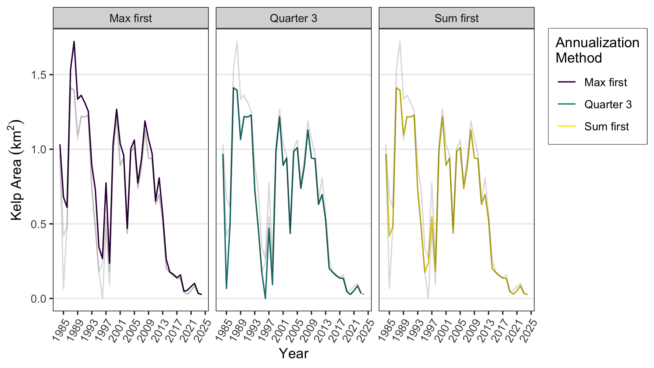

plot of chunk time_series_plot_comparison

Kelp status

The status of kelp segments can be computed relative to the historical baseline (1984 - 2013) with the get_kelp_status() function. This function uses the computed time series and kelp presence data frames from the extract_time_series() and get_kelp_presence() functions, respectively. Individual kelp segments or subsets of kelp segments may be specified with the segment_id argument, and the desired year may be specified with the status_year argument. The function will return the status for all segments if segment_id = NULL (default) or for the latest year in the Landsat data if status_year = NULL (default).

Status is calculated by dividing the given year’s kelp area by the historical median across 1984-2013 for each kelp segment. A value of -999 indicates that there is not enough data to determine a status for the given kelp segment.

kelp_status_2020 <- get_kelp_status(
  annual_time_series = sum_first_annual_ts,
  kelp_presence = kelp_presence,
  status_year = 2020
)

kelp_status_2020
#> # A tibble: 311 × 3
#>    Segment_ID  year  status
#>    <chr>      <dbl>   <dbl>
#>  1 CA_1        2020  128.  
#>  2 CA_10       2020    1.90
#>  3 CA_100      2020    2.23
#>  4 CA_101      2020    6.41
#>  5 CA_102      2020    2.23
#>  6 CA_103      2020 -999   
#>  7 CA_104      2020   26.2 
#>  8 CA_105      2020 -999   
#>  9 CA_106      2020 -999   
#> 10 CA_107      2020 -999   
#> # ℹ 301 more rows

kelp_status_CA_70 <- get_kelp_status(
  annual_time_series = sum_first_annual_ts,
  kelp_presence = kelp_presence,
  segment_id = "CA_70"
)

kelp_status_CA_70
#> # A tibble: 1 × 3
#>   Segment_ID  year status
#>   <chr>      <dbl>  <dbl>
#> 1 CA_70       2024   2.88